MATLAB Introduction
Introduction to Matlab
This section will introduce you to the Matlab numerical computing environment. If you have some experience with other computer languages, you can probably get by with just a quick skim of this section. You can pick up most of what you need just by following the examples. If you have little or no experience, type along as you read. This section is written to accompany the Error Analysis Exercise (EAX) and other Physics 111 Advanced Lab experiments that need data analysis completed.
If you would like a more formal introduction to Matlab, try visiting this link at the Mathwork's website and click on 'Introduction'. The first few sections are particularly helpful.
At the end of this page, you should know how to:
- Run Matlab and change the working directory
- Create a variable and assign it a value
- Call functions and do basic math operations
- Work with numerical matrices
- Work with cellular matrices
- Create a basic plot
Don't worry if you have a little trouble with some of the concepts in the section. Things will become clearer as you do the examples in the following sections.
About Matlab
The name 'Matlab' is short for 'Matrix Laboratory'. Matlab is programmed in a language called m-code. M-code was originally created in the 1970s as a simple alternative to Fortran. Since that time, The Mathworks (the company that develops Matlab) has added many new features to the language. Matlab contains sophisticated functions for manipulating matrix data. A student license to Matlab is available for about $100. Physics 111 has Matlab with Statistics Toolbox package installed on all lab computers; see lab staff for remote access.
Prepare Your Environment
The first step is to copy any data or other files with Matlab scripts to your own My Documents directory.
Launch Matlab inside 111-Lab
Now launch Matlab from any 111-Lab computer. From the Start menu, select: All Programs->Matlab R2008b->Matlab R2008b
No More Remote Matlab from outside of the 111-LAB
There is no remote access to Matlab. Use it from within the Physics 111-Lab or purchase your own student copy for home use.
Change Working Directories
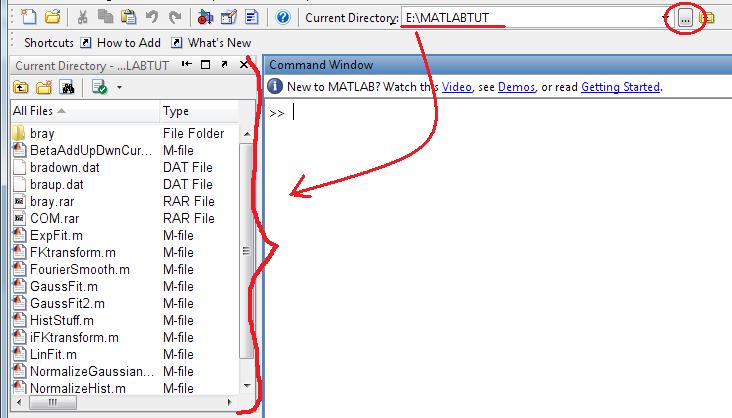
Before you start typing commands, change the current working directory to your own My Documents folder. To do this, click on the little button with three dots near the top right of the Matlab window. Use the Windows directory browser that comes up to select the folder you want. Scroll to the top and select My Documents and then select a working folder Your experiment Name.
Note that any scripts you wish yo use must be placed in this folder to ensure they work properly! It also provides quick access to your data for importing purposes (as we will discuss later).
Entering Commands
The Matlab window is divided into multiple panes. By default, on the top left is a listing of the current directory. Below that is a history of the commands you have typed. On the right is the command window. Click anywhere inside the command window to select it. Further to the right is the Workspace, where your variables are listed.
Matlab in an interpreted language. To enter a command, just type it at the prompt in the Command Window. In this document, commands are shown with a gray background. After each gray section, the output of the commands is shown, like this:
>>2 + 3

ans =
     5
A good parallel to MATLAB's command window is the starting screen of a standard graphing calculator. You type in a command, and then the program evaluates your command. In the example above, we are performing simple addition. Another example:
>>sin(1.2)

ans =
     0.9320
Here we evaluate the sine of 1.2 radians, using the predefined function "sin".
Note that if you wish for Matlab to evaluate an expression but NOT display the result on the screen simply put a semi-colon at the end of the line.
>>sin(1.2);
This might not seem useful if you're not actually doing anything with that result since you can't see it, but when you save something into a variable (we shall discuss this promptly) or are performing a manipulation on a large amount of data, you might not want the screen to be suddenly filled with the result of your expression.
Getting Help
Type help and the name of the command to get full documentation. If you are really in trouble, try help help.
>> help sin
 SIN    Sine of argument in radians.
    SIN(X) is the sine of the elements of X.

    See also asin, sind.

    Overloaded methods:
       distributed/sin

    Reference page in Help browser
       doc sin
Create Some Variables
In Matlab, variables are dynamically created and typed. This means you can create a new variable just by typing its name and setting it equal to a value. For example:
>>favoriteNumber = 7

favoriteNumber =
     7
>>favoriteColor = 'yellow'

favoriteColor =
     yellow
Accessing these variables is just as easy. Just use the name that you gave it in a new command and Matlab will use the stored value:
>> favoriteNumber + 2

ans =

     9
If you ask Matlab to evaluate an expression but don't store it in a variable (as we did above with favoriteNumber + 2) then Matlab automatically stores it in the variable "ans". This can be referenced again in another command:
>> ans + 3

ans = 12
However, note that the previous value of ans has been overwritten with the new one since we again did not supply a variable to store it into. Remember to store important data values in variables!
Also note that all your variables are displayed in the Workspace pane of the Matlab screen. These variables can be easily copied/renamed here.

The Matlab Workspace contains all the variables in this session of Matlab. |
Entering a Numerical Matrix
Matlab makes it easy to create matrices. For example, to create a one dimensional matrix, separate the elements by commas or spaces. Use a semicolon to delimit the rows of a two dimensional matrix
>>fib = [ 1, 1, 2, 3, 5, 8, 13 ]

fib =
     1     1     2     3     5     8    13
>>sudoku = [5 3 4 6 7 8 9 1 2;
            6 7 2 1 9 5 3 4 8;
            1 9 8 3 4 2 5 6 7;
            8 5 9 7 6 1 4 2 3;
            4 2 6 8 5 3 7 9 1;
            7 1 3 9 2 4 8 5 6;
            9 6 1 5 3 7 2 8 4;
            2 8 7 4 1 9 6 3 5;
            3 4 5 2 8 6 1 7 9 ]

sudoku =
     5     3     4     6     7     8     9     1     2
     6     7     2     1     9     5     3     4     8
     1     9     8     3     4     2     5     6     7
     8     5     9     7     6     1     4     2     3
     4     2     6     8     5     3     7     9     1
     7     1     3     9     2     4     8     5     6
     9     6     1     5     3     7     2     8     4
     2     8     7     4     1     9     6     3     5
     3     4     5     2     8     6     1     7     9
Some Useful Matrix Generation Functions
The ones and zeros functions generate matrices of given dimensions. For example:
>>someOnes = ones(1,10)

someOnes =
     1     1     1     1     1     1     1     1     1     1

>>someZeros = zeros(3,3)

someZeros =
     0     0     0
     0     0     0
     0     0     0
Generating Sequences of Numbers
Use the colon (:) operator to generate a matrix of uniformly incrementing values. With two operands, each element increases by 1. With three operands, each element is incremented by the middle value.
>>1:10

ans =
     1     2     3     4     5     6     7     8     9    10

>>1:.2:2

ans =
    1.0000    1.2000    1.4000    1.6000    1.8000    2.0000

>>2:-.2:1

ans =
    2.0000    1.8000    1.6000    1.4000    1.2000    1.0000
Accessing and Editing the Elements of a Matrix
Unlike most other computer languages, index values in Matlab start with with 1 (not 0). For example, the fourth element (index = 4) of fib is 3, while the sixth element (index = 6) is 8. To access an individual element of a matrix, use the parenthesis operator like this:
>>fib(4)

ans =
     3

>>fib

fib =
     1     1     2     3     5     8    13
Note in this example that we only defined fib to 7 elements. Asking fib for an 8th element would result in an error, but we can still assign an 8th element to the matrix and Matlab will dynamically resize it:
>>fib(8) = 21

fib =
     1     1     2     3     5     8    13    21
Multi-dimensional matrices are accessed using the same parenthesis operators, but with the index of each dimension followed by commas. As an example, in a 2-dimensional matrix, variable(row,column) accesses the row-th, column-th element of variable.
>>sudoku(3,3)

ans =
     8
To access multiple elements of a matrix, use a : in the matrix to denote the range of selection. For example, to get the 1st through 9th elements of the first row in sudoku:
>>sudoku(1,1:9)

ans =
     5     3     4     6     7     8     9     1     2
You can also simply use a : without any numbers to denote "all" of a column or row.
>>sudoku(:,3)

ans =

     4
     2
     8
     9
     6
     3
     1
     7
     5
Matricies can be used as elements in new matricies to combine them with other ones. As an example, if we had 2 matrices of numbers that we wanted to append to one another:
>> A = 1:10

A =

     1     2     3     4     5     6     7     8     9    10

>> B = 11:20

B =

    11    12    13    14    15    16    17    18    19    20

>> AB = [A B]

AB =

  Columns 1 through 14

     1     2     3     4     5     6     7     8     9    10    11    12    13    14

  Columns 15 through 20

    15    16    17    18    19    20
Note that we combined A and B using [A B] This results in the two matrices being placed in a row. If we used a semi-colon instead of a space the two matrices would be placed in a column:
>> AB = [A ; B]

AB =

     1     2     3     4     5     6     7     8     9    10
    11    12    13    14    15    16    17    18    19    20
Basic Mathematical Operations
Basic math operations in Matlab are simple. Almost all of the operations that work on single numbers will also work on matrices. Some examples:
>>favoriteNumber * 3

ans =
    21

>>fib * 3

ans =
     3     3     6     9    15    24    39    63

>>fib + 3

ans =
     4     4     5     6     8    11    16    24

>>fib(2:5) * 3

ans =
     3     6     9    15

>>sum(sudoku(1,1:9))

ans =
     45

>>mean(sudoku(1,1:9))

ans =
     5
Some notes should be made however. In order to raise a number by a power, you use the ^ operator (i.e. 2^3 = 8). Saying A^2 will however perform the procedure: A*A which would be matrix multiplication. If you want to say, raise the power of every element by 2, use a . before the operator. Examples:
>> A

A =
     1     2     3     4     5     6     7     8     9    10

>> A^2
??? Error using ==> mpower
Matrix must be square.

>> A.^2

ans =
     1     4     9    16    25    36    49    64    81   100

>> B

B =
    11    12    13    14    15    16    17    18    19    20

>> A*B
??? Error using ==> mtimes
Inner matrix dimensions must agree.

>> A.*B

ans =
    11    24    39    56    75    96   119   144   171   200
Note the final example. Here we use the .* operator to multiply each element of A by each element of B.
Many of the predefined functions in Matlab are designed to take a matrix and output a matrix that is the result of applying the function to each element in the matrix. As an example:
>> sin(AB)

ans =

  Columns 1 through 8

    0.8415    0.9093    0.1411   -0.7568   -0.9589   -0.2794    0.6570    0.9894
   -1.0000   -0.5366    0.4202    0.9906    0.6503   -0.2879   -0.9614   -0.7510

  Columns 9 through 10

    0.4121   -0.5440
    0.1499    0.9129
Importing Data

Importing Data through the Current Directory Pane
The newer versions of Matlab with their nice graphical user interface have made it very easy to import data. If you have your data in your working directory you can just right-click the file in the directory browser pane and click Import Data to start the Import Data wizard. If your data is stored outside of the working directory, clicking File-> Import Data will bring up a Windows file browser window where you can select your data file.
The Import Wizard - 1
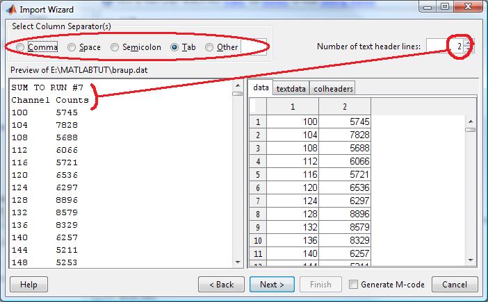
At the left side of the Import Wizard is a display of your data file you are importing. Make sure that the number of header lines in your text file is correctly input in the box at the top-right of the wizard! An incorrect number of header-lines could result in loss of data or incorrect formatting. Also ensure that Matlab knows how columns are separated in your data file (i.e. different data values on the same line are separated by tabs, spaces, commas, etc.) A preview of what the variable will be is shown on the right side.

The Import Wizard - 2
On the next screen will be a display of the variables that will be imported. By default Matlab will select to "Create variables matching preview." which references the preview from the previous window. If you are using this setting (and most of the time it is useful to) the default variable-names shown are typically colheaders, data, and textdata. colheaders and textdata represent Matlab's attempt to use the text header lines to extract information about the data and can be typically ignored (Just make sure that you know for yourself which column in your data variable represents what!) The data variable always defaults to the name data, so if you're importing multiple data-sets, ensure that you rename the variable to something that you will be able to differentiate between.
Now that you have your data variable, you can use it as a matrix as described in the preceding sections. As a tip, it might be easier for you to reference the data if you separate it out of the 2-dimensional array. In our example, the data we were importing was a histogram, where the first column was the channel and the second was the corresponding number of counts.
>> channels = braup(:,1);
>> counts = braup(:,2);
This gives us two separate 1-dimensional matrices, which are more commonly used by the plot and fitting functions described later. Note that we used a colon instead of a row number to denote that we wanted all rows (i.e. the entire column). Also note that we used a semi-colon at the end of the expressions to suppress output in order to ensure that the Command Window was not suddenly filled up with 976 rows of data.
Of course we could always just use variable(:,1) for example to get the 1st column of a multi-dimensional matrix for plotting, but sometimes using separate variables can make it less confusing. Do note that by doing this we essentially doubled the space used by the variables in memory (since it is saved twice now, as a multi-dimensional matrix and as two separate 1-dimensional ones), so keep that in mind if your space is limited.
Matlab Data Structures
Sometimes, it is useful to group related pieces of data together. Matlab supports data structures with the dot (.) operator. Note: Matlab likes to print a bunch of junk out after most commands. To suppress this sometimes annoying habit, put a semicolon after the command. This is particularly useful when you are working with large matrices. Begin comments in your code with a % character as below.
For example:
Fred = struct();        % creates an empty structure
Fred.height = 182;
Fred.weight = 72;
Fred.hatSize = 58;
Fred.favoriteColor = 'gray';

>>Fred

Fred =

           height: 182
           weight: 72
          hatSize: 58
    favoriteColor: 'gray'
Fred's height in inches is:
>>Fred.height / 2.54

ans =

   71.6535
Cellular Matrices
Matlab supports another kind of matrix called a cellular matrix. Instead of numerical values, each element in a cellular matrix can hold any Matlab type. Elements of cellular matrices are accessed with braces instead of parenthesis.
cellMatrix = { }            % creates an empty cellular matrix
cellMatrix{1} = fib;
cellMatrix{2} = sudoku;
cellMatrix{3} = Fred;

2.54 * cellMatrix{3}.height

ans =
     462.2800
About your variables
The whos command prints a list of all the defined variables with details about their size and type.
>>whos

Name                 Size                    Bytes  Class

  Fred                 1x1                       528  struct array
  ans                  1x1                         8  double array
  cellMatrix           1x3                      1420  cell array
  favoriteColor        1x6                        12  char array
  favoriteNumber       1x1                         8  double array
  fib                  1x8                        64  double array
  someOnes             1x10                       80  double array
  someZeros            3x3                        72  double array
  sudoku               9x9                       648  double array

Grand total is 230 elements using 2840 bytes
Loops
A for loop executes a sequence of commands multiple times. The loop begins with a for statement and ends with an end statement. The for statement specifies an index variable and an ordered set of values (contained in a matrix). The statements in the body of the loop are executed one time for each of the possible values, in order. For example, the body of the following loop executes 10 times and calculates the sum of the first 7 positive integers.
s = 0;
for i = 1:7
    s = s + i
end

s =
     1

s =
     3

s =
     6

s =
    10

s =
    15

s =
    21

s =
    28
This loop calculates the sum of the the odd integers between 1 and 7:
s = 0;
for i = 1:2:7
    s = s + i
end

s =
     1

s =
     4

s =
     9

s =
    16
Plotting Data
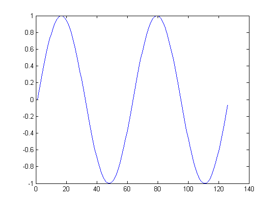
The plot function opens a graphics window and plots its arguments. The statement plot(y) (with one argument) plots the columns of y versus their index. For example:
x = -2*pi:.1:2*pi;
y = sin( x );
plot(y);
More Plotting Options
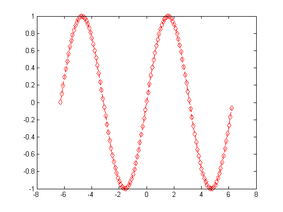
If x and y are vectors, plot(x,y) plots vector y versus vector x. Notice the difference in the x axis. The third (optional) argument to plot is a line specification. This particular string of characters will create a red (r) dashed(--) line with diamond shaped (d) markers at each data point. There are many more options available for the plot command. Type help plot for details.
plot(x, y, 'rd--');
More Advanced Features
Input and Output
Matlab supports C-like syntax for file I/O. To open a file for reading, use fopen command (type help fopen in the command window to display the syntax)
f = fopen('MUO_Calib_raw.txt','r');
fopen returns the file handle f, which is used in subsequent I/O operations, e.g. reading.
To read a formatted files, e.g. a set of space- or tab-delimited values, use fscanf function:
[data,count] = fscanf(f,'%f %f %f %f %f',[5,inf]);
This fill read the entire file f, and convert the contents into a 5*inf matrix data of floating-point values. count contains the number of values read, i.e. 5 times the number of columns in the matrix data. A more powerful function to use is textscan (see help textscan) which would allow you to skip headers, etc. It returns a mix-typed cell structure, which can be converted to a matrix with function cell2mat.
To store some data in a file, you can use the following snippet:
of = fopen('junk.dat','w');
fprintf(of,'%9.3e %6.4f %9e %6.4f %9.3e\n',data(:,1:10));
fclose(of);
This will write 10 formatted lines of data.
Plotting Data
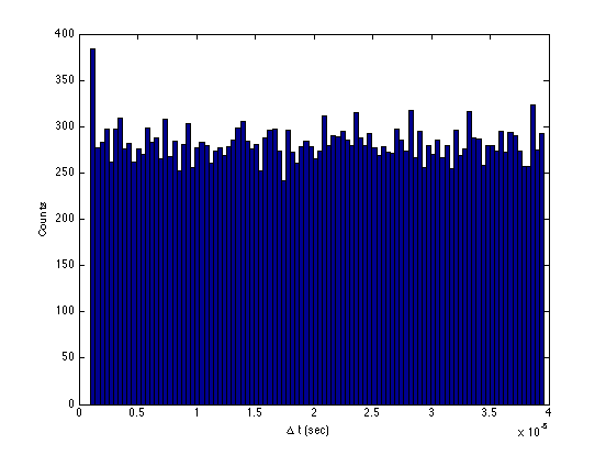
You can make a histogram, i.e. a binned distribution of data, using hist function:
hist(data(1,:),100);
xlabel('\Delta t');
xlabel('\Delta t (sec)');
ylabel('Counts');
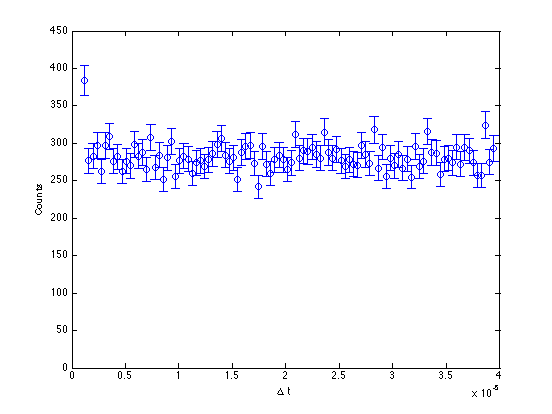
It would be appropriate to plot the data with error bars, to reflect statistical fluctuations. Unfortunately, unlike ROOT package (see Muon Analysis in ROOT), Matlab will not do this for you automatically. Fortunately, this means you have to think about what you are doing.
[h,dt] = hist(data(1,:),100);   % returns vector of y-values and x-values
e = sqrt(h);                    % computes Poisson errors for each bin
errorbar(dt,h,e,'o');           % plots the graph with error bars
axis([0 4e-5 0 450]);           % resets axis limits
xlabel('\Delta t');             % adds labels
ylabel('Counts');
Fitting
Simple, polynomial fits can be done with polyfit command:
[fitres,S] = polyfit(dt(2:100)*1e6,h(2:100),1) % least-squares 1st-order poly fit h vs dt. Notice rescale of x axis

fitres =

    0.0285  280.3845


S =

        R: [2x2 double]
       df: 97
    normr: 155.5413
The fit returns the coefficients (p1 and p0, from highest power to lowest), and a structure S that can be used to compute the uncertainties in the parameters, and other useful information:
cov = (inv(S.R)*inv(S.R)')*(S.normr^2)/S.df % covariance matrix for poly coefficients

cov =

    0.0207   -0.4241
   -0.4241   11.2174

sqrt(diag((inv(S.R)*inv(S.R)')*(S.normr^2)/S.df)) % coefficient errors

ans =

    0.1438
    3.3492
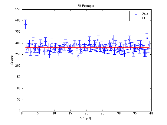
Now you can plot the fit on top of the data:
data_handle = errorbar(dt*1e6,h,e,'o');  % rescale x axis
axis([0 40 0 450]);
xlabel('\Delta t (\mus)');
ylabel('Counts');
title('Fit Example');

hold on
fit_handle = plot(dt*1e6,fp,'r-');  % plot values of the fit on the same plot
legend([data_handle;fit_handle],'Data','Fit');
hold off
The problem with polyfit is that it implements unweighted least-squared minimization. To do a weighted fit, e.g. to weight the points by their inverse variances, you can use lscov function, or (instructive) implement your own algorithm based on formulae in Taylor. Those who want an easy way out can download one of the functions freely available on the internet. For instance, the algorithm for a weighted linear fit can be found here.
Additional Packages
Phys111 installation of Matlab includes the Statistics Toolbox, which provides advanced statistical functions, including distribution fitting, etc. Type "doc" in the command window and then navigate to "Statistics Toolbox" in the right-hand menu. Of particular use is the interactive "Distribution Fitting Tool", which you start by typing
dfittool
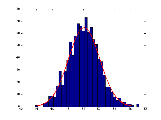
in the command window. The functionality is also accessible through the command line. The following snippet shows an example of an unbinned maximum-likelihood gaussian fit:
rdata = normrnd(50,2,1000,1); % generate 1000 events, Gaussian-distributed with mean=50 and sigma=2
[m,s,mci,sci] = normfit(rdata,0.32) % fit to a Gaussian; returns mean, sigma, and 68% confidence intervals

m =

   50.0888


s =

    1.9996


mci =

   50.0258
   50.1517


sci =

    1.9566
    2.0456

mci-m  % + and - errors on mean

ans =

   -0.0629
    0.0629

sci-s  % + and - errors on sigma

ans =

   -0.0430
    0.0460
histfit(rdata,40)  % plot results
Unbinned ML fits are generally more powerful than binned, least-squares fits, but you have to be careful with the outliers in the data. ML fits also do not provide an immediate goodness-of-fit measure, such as \( \chi^2/df \), so you have to compute it after the fact for a reasonably binned histogram. For a ML fit tool, type help mle.