Design and Documentation (QIE)
Quantum Interference and Entanglement Lab
This lab was developed by Berkeley Professor Hartmut Haeffner and several undergraduate students and volunteers (see acknowledgements). The current experiment is to show a violation of Bell's inequalities. Our next goal is to add a Mach Zehnder interferometer and/or Hong-Ou-Mandel interferometer to the experiment. By fully shielding the blue laser beam path, which is set up permanently, we can allow students to assemble and align all optical components downstream of the BBO crystal. A set of detection arms with attached breadboards that pivot at the BBO crystal makes it easy for students to adjust the angle at which downconverted photons are detected without the tedium of moving each optical component separately.
Acknowledgements
During the summer of 2011, assembly began led by Segre intern Will Morong, with help from another intern, Bennett Sodergren. During the 2011-2012 academic year two physics undergraduate students, Kelsey Johnsen and Sachi Wagaarachchi, continued the development with Professor Haeffner, and observed violation of the Bell's Inequality on April, 2012. In the summer of 2012, Segre interns Nitin Egbert and Griffin Hosseinzadeh continued to improve the experiment, and wrote the Wiki writeup for the students to use. The experiment was successfully tested by the third Segre intern, Harry Nunns. Tom Andrade contributed several custom fabricated components, including the BBO mount, rotating arms/breadboards, and the power supply/heat sinks for the single photon detectors. This experiment is constantly upgraded and maintained by Don Orlando.
Funding for this experiment has been provided by an NSF Grant to Hartmut Haeffner and a generous donation by alumnus Hans Mark.
Apparatus
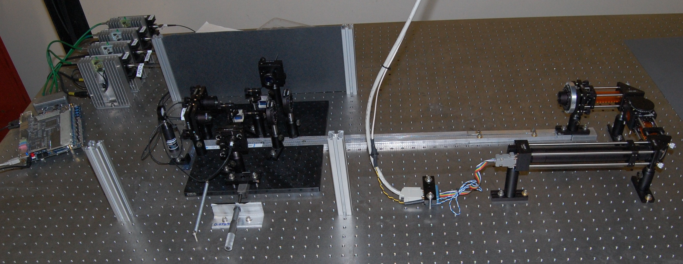
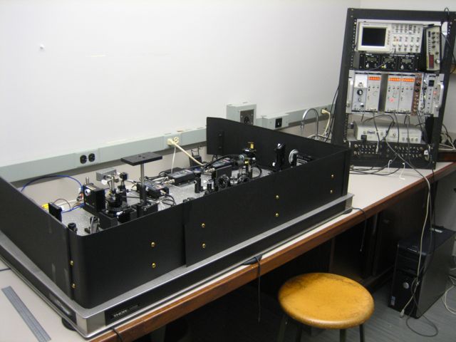
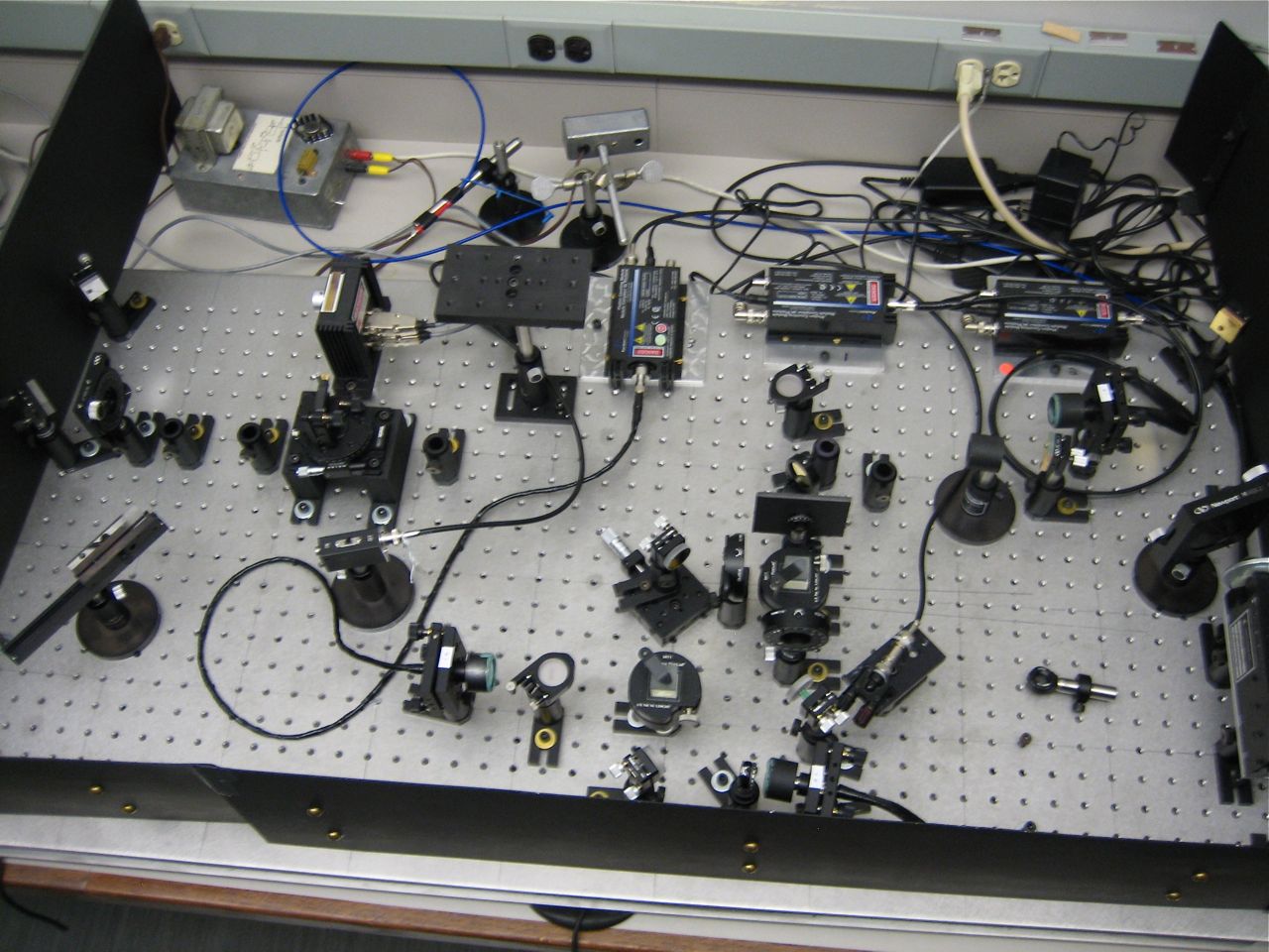
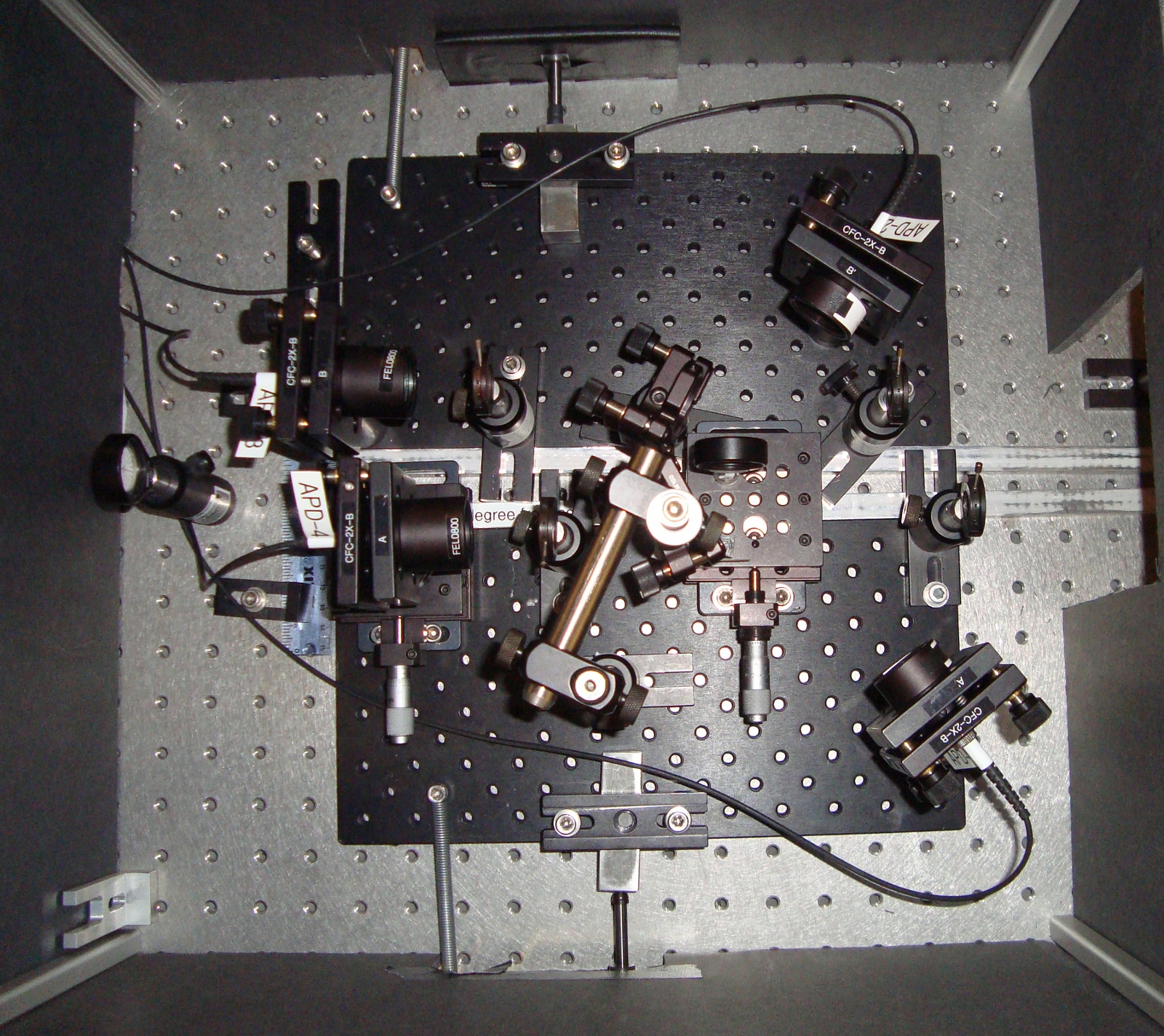
QIE apparatus: blue laser path (right), detection arms with attached breadboards (left center), FPGA card and 4 APDs (far left). When students do the experiment, they build and align all optics on the detection arms. The blue laser beam path is fully shielded and remains set up permanently.
Blue Laser Beam Path
Our laser is a 405 nm Blu-Ray laser diode running at 100 mA and a power of about 20 mW at the BBO crystals (a fraction of what it actually produces). This is connected to a cage that contains: a short-focus lens (4.5 mm) for collimating the laser beam, a long-focus lens (40 cm) for finely adjusting the focus, a steering mirror, a half waveplate, a 405 nm bandpass filter, the second steering mirror, and then the BBO crystals. The first steering mirror centers the beam on the crystals, while the second one adjusts its angle so that it is 2.5 degrees away from each detector and roughly level with them. For this, the distance between the mirrors should be greater than the distance from the second mirror to the BBO crystals.
The half waveplate will be adjusted using the coincidence counts to give an equal superposition of vertical and horizontal laser light. Each BBO crystal downconverts a photon with a polarization along a particular axis to two photons of the same polarization (opposite to what the laser beam was). Our setup has two BBO crystals with their conversion axes orthogonal to each other, so that one downconverts horizontally polarized light and the other yields a vertically one. The downconverted photons from each of these emerge in cones roughly 2.5 degrees off the laser-beam axis. Actually, if you look at other angles you will still see downconverted photons, but in this case the photon pairs come at different angles and energies, while three degrees is the point at which they are degenerate.
Downconverted Photon Beam Path
Because each of the BBO crystals emits light of the same energy in cones that overlap, a detector placed in the appropriate position has a nearly equal chance of seeing horizontally and vertically polarized downconverted photons. Moreover, until some sort of measurement of polarization is applied to the system, the two types of photons are indistinguishable. Because of this, according to the rules of quantum mechanics, these photons are in a superposition of the two possibilities- the possibility of a pair of horizontally polarized photons or a pair of vertical ones. This makes the photons entangled. To understand this, it is helpful to think of the double-slit experiment. In that setup, we said that particles arriving at the screen could have come through the left or right slit, so in fact until measured they exist in a superposition of the two. There are two differences to keep in mind, however. The first is that in the double slit experiment, these two possibilities interfere constructively and destructively at different points on the screen, producing fringes, but in our entanglement setup we keep the phase relationship between the paths constant. This is rather like if you imagine shrinking the double-slit screen until it only covers the central bright fringe. The second is that our two possibilities now correspond to two particles, not one, which is why this system is entangled.
Now then, these entangled photons arrive at the two branches of our detector setup. Each branch has an iris, a half-waveplate, a polarizing beam splitter cube, and two lenses at either face of the cube, which are protected by 800nm low-pass filters and feed collected photons through fiber optic cables to a total of four Avalanche Photodiode (APD) single-photon detectors. The irises and filters help to minimize noise from other photons. The waveplates and beamsplitters, meanwhile, allow us to measure each photon of the pair along any polarization axis. The waveplates rotate the photon polarizations, which is equivalent to rotating the detector basis in the other direction, and the polarizing beam splitters do the actual job of separating out the different polarizations- and thus collapsing the quantum state.
Single Photon Detectors and Coincidence Detection
Our APDs can detect anywhere between a few hundred to about 30 million photons per second, and put out a voltage pulse for each one. The pulses from the four APDs pass to the next part of the signal processing chain, the DE-2 FPGA. An FGPA (Field-Programmable Gate Array) is essentially a hardware circuit that is configured by software. Instructions, written in a language called VHDL, are loaded onto the machine that tell it what gates and modules to route incoming signals through, and how to output results. The software we've loaded onto ours allows it to count up the single pulses, count coincidences between any set of detectors within four possible time windows, and stream all of this to our computer's Labview program. The FPGA streams eight registers of running counts to the computer. The first four are the counts on detectors A, B, A' and B' (in that order), and the last four are coincidence counts that are determined by flipping switches on the front of the device. Each register has four switches, one for each detector, and one simply flips the ones for the detectors that one wishes to include in the coincidence count, allowing for 2, 3, or 4-fold coincidences as desired. To measure Bell's inequality we have the registers set to measure AB, AB', A'B, and A'B' coincidences, respectively. The last two switches on the FPGA toggle between four possible settings for the allowed time window of coincidence. For 0 as off and 1 as on, the settings are:
00- length of incoming pulse (~20 ns)
01- roughly 15 ns
10- roughly 10 ns
11- roughly 5 ns
All these time values drift perhaps ±3 ns with temperature and how the DE2-115 is feeling today.
Explanation of how the coincidence window settings work: Coincidence detection is just done by putting two or more pulses through an AND gate. If they overlap enough to put out an output pulse (and it appears that no more than 1 ns is required for this), they count as a coincidence. Therefore, narrowing the coincidence window is done by shortening the pulses- if pulses are sufficiently delayed, once they are shortened they will no longer overlap and so will no longer produce a coincidence pulse. The shortening is done by ANDing a pulse with another version of the pulse that is slightly delayed and inverted. The output is zero except for the time between when the first pulse and delayed pulse arrived. Because the delay must be very short, less than even one cycle on the DE-2's 50-MHz clock, the delay is a hardware delay. A copy of the pulse is essentially routed through a few buffers, which each take a nanosecond or two, before being inverted and sent through an AND gate with the original.
Running counts from the 8 registers are streamed at 10 Hz to the computer, which when running the appropriate labview program will add them all up for a user-defined time, display the result, and record data.
Note: VHDL and Labview provided by Mark Beck, beckmk[at]whitman.edu .
Sketch of the quantum state evolution of the system:
Light from the laser: $|\psi\rangle= \cos \phi |H_{las}\rangle + \sin \phi |V_{las}\rangle $, where $\phi$ is some unknown angle.
First waveplate: $|\psi\rangle=\frac{1}{\sqrt{2}}(|H_{las}\rangle + |V_{las}\rangle) $
BBOs: $|H_{las}\rangle \rightarrow |V_1V_2\rangle$, $|V_{las}\rangle \rightarrow |H_1H_2\rangle$
$|\psi\rangle=\frac{1}{\sqrt{2}} (|H_1H_2\rangle + |V_1V_2\rangle)$ (laser photons are downconverted into two photons of half the frequency and the opposite polarization).
Passing detector waveplates set to $\alpha$ and $\beta$ from the horizontal:
$|\psi\rangle=\frac{1}{\sqrt{2}}\lbrace(\sin\alpha\sin\beta+\cos\alpha\cos\beta)|V_1V_2\rangle $
$+ (\cos\alpha\sin\beta-\sin\alpha\cos\beta)|H_1V_2\rangle $
$+ (\sin\alpha\cos\beta-\cos\alpha\sin\beta)|V_1H_2\rangle $
$+ (\sin\alpha\sin\beta+\cos\alpha\cos\beta) |H_1H_2\rangle\rbrace $
Passing through the beamsplitters acts as a measurement of polarization along the H-V basis, collapsing the state into one of these eigenstates.
Equipment Notes
Single Photon Detectors
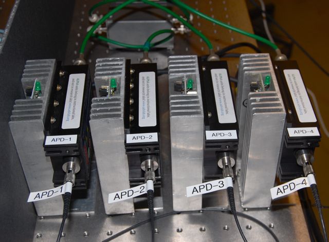
We use the Educational Use Single Photon Counting Module SPCM-EDU CD3375 from Excelitas Technologies (formerly Pacer). This set of 4 avalanche photodiodes (APD) is available only through bulk purchases arranged by ALPhA and AAPT for use in educational settings.
Fiber optic cables to use as input to the APDs were obtained from Pacer/USA, part number SPCM-QC9. Standard fiber optic cables from Thorlabs were not workable due to light leakage.
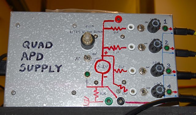
To power the 4 APDs, we use a Power-One 5V/3A linear power supply with over voltage protection. We enclosed this in a box with fuses and LED indicators (see photo below). We mounted each APD on a heat sink with LED indicator as an extra precaution to avoid damage by overheating if students leave the power on with the fiber optic cable disconnected. The APDs have some circuitry to prevent damage from excess light, but this could be defeated if the unit overheats.
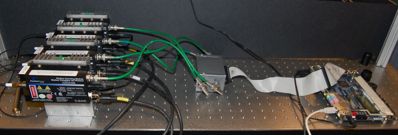 APDs on left send data to FPGA card on right |
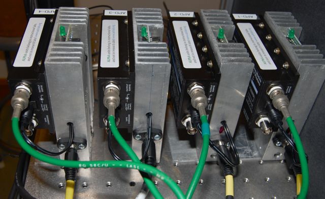 Power in and data out from APDs |
Using the LabVIEW Program
Our LabVIEW program makes it quite simple to measure S for Bell's Inequality. The program is currently located at C:\QIE\QIE_Labview 2012\Bell_rs232(mod).vi. This is a stripped-down and heavily modified version of the Labview program Bell_rs232.vi we got from Mark Beck. The original labview program and its documentation are contained at C:\QIE\CCM\Beck Labview Programs. The documentation of this program contains many descriptions of settings that are now obsolete for our version, but the descriptions of what we still have are all valid.
As of June 2012, all the LabVIEW files necessary for student use have been compliled into a LabVIEW library, C:\QIE\QIE_Labview 2012\QIE_Counter.llb. Students should open this library and run Bell_rs232(mod).vi. The most recent version displays count rates on each thermometer, while still showing raw counts in an array indicator on the side. Students can see the count rates change in real time over short update periods. Two functions are present for data taking: a "Take Snapshot" button, which takes a single sample for up to 200 seconds and records settings and comments, and a "Take Data" button which takes multiple samples and calculates values for the specified experiment.
Here are descriptions of the buttons and displays on our LabVIEW program:
8 Thermometers with count rates, labelled A, A', B, B', AB, A'B, AB', A'B': these are the counts the program reads from the DE2-115. The first four are the counts on each detector divided by the update period, the second four are coincidence counts between detectors divided by the update period. The labels on the second four are only valid if the switches on the DE2-115 are set to display the corresponding coincidences; if we are only doing Bell inequalities there is no need to ever change these anyway.
E and E-meter: This automatically calculates E for the given four coincidence counts. It simply adds the fifth and eighth registers, subtracts from this the sixth and seventh, and then divides all this by the sum of these four counts. If the two half waveplates are set at one of the correct pairs of angles for Bell Inequality testing, this gives you one of the four values that are added together to get S. For reference, the four angle pairs are E(-45,-22.5), E(-45,22.5), E(0,-22.5), E(0,22.5), with the second one negative. These are polarization angles, not waveplate settings.
Subtract Accidentals and Coincidence Resolution: Subtract accidentals, if turned on, subtracts the statistical number of chance coincidences from the four coincidence counts, calculated using the individual counts on each detector and the coincidence resolution (or time window), entered in the four numerical inputs.
Round Counts in Display: Simply rounds the count rates in the display to remove confusion from reading decimals.
Data Taking Controls: You can set the update period for data taking, and the number of samples at each angle. After specifying the experiment that you are going to be performing and clicking "Take Data," the program will tell you what angles to set the half wave plates, take samples at each angle, and calculate various experimental results from the data.
Two things to keep in mind if you want to turn this on:
1. You should probably measure your coincidence windows first, since they have a tendency to drift. Use a pulse generator set to 15ns 2.0V pulses, and slowly increase the delay between pulses starting at 1 ns until you measure no coincidences.
2. Since accidental coincidences can only reduce your S-value, if you are already comfortable violating the inequality this is probably not worth it.
Counter Port: which computer port you are looking for data over. Should be set to COM1.
Status: what the program is doing. Pretty much obsolete now, because when it is running the answer is always 'reading counters.' A holdover from the original program, which would also stop reading data sometimes to move motors that controlled the waveplates.
Data taking parameters: these are the settings for when you enter data taking mode, in which the program writes all the counts to a text file. The program will count for the input time, and the input number of samples, over each of the four angle combinations. This means the total time taken is 4*time*samples.
Known error: occasionally, the LabVIEW program will crash when you try to run it, complaining that it cannot access the VISA port or the connection timed out, and also annoyingly opens up the file for the close-session sub-vi. Usually, it will work if you just try running it again. It will also give similar errors every time you try to run the program with the DE2-115 turned off. If you are unable to connect to the DE2-115 despite powering it off and powering it back on, the proper procedure is to turn off the DE2-115, then restart the computer, and power the DE2-115 back on after the computer has restarted and you are logged in. For reasons unknown, Windows occasionally grabs the serial port and refuses to relinquish it to LabView if the DE2-115 is turned on during startup.
Viewing/Loading a Program on the DE2-115
Start by double-clicking on the main program file for our program, which is called "RS232coincidencecounter.qpf". This is currently found at C:\QIE\CCM\DE2_RS232_CCU_Q72\RS232coincidencecounter.qpf on the computer in the QIE room. This should open Quartus II, the software used to edit, compile, and load programs onto the DE2-115. Once Quartus II launches, you should see a blank main screen, and a few smaller windows. In the top left under Entity our FPGA is listed, the Cyclone IV E, and below that the icon for "RS232coincidencecounter". Double-clicking on this brings up the VHDL code for the top-level program, which can be inspected. This file also references 7 smaller auxiliary files, which are listed in the "files" tab just below that window.
Once any changes have been made, the program can be compiled by clicking on the little purple triangle named "Start Compilation" at the center of the upper toolbar. The compilation and some optimizations will run, and it will either compile successfully or return an error. If it complies successfully you may still get a ton of warning messages (ie around 900); most of those will be of no consequence.
If you modify inputs or outputs, you may need to assign or change pin settings on the DE2-115. This controls where the program's input and output signals are actually expressed on the chip- for example, the input signals for the detector counts are wired to four pins on the 40-pin header, while the output signals for the switch indicators are wired to the 17 red LED lights so that they show when the switches are flipped. This is located under Assignments>Pin Planner. Here there is a great big list of all the inputs and outputs on the DE2-115. All of them will be shown as "Assigned", meaning they have a name/signal attached to them, but the vast majority will be listed as having a direction of "unknown", which means they are not actually used by our design. To assign a pin, first look up the name of the particular input or output you want. These are listed and described in the DE2-115 user manual, which is on the CD that came with the device or on the QIE computer at "C:\QIE\References\DE2_115_User_manual.pdf". Once you look up this pin, find it in the Pin Planner window and then either change the name of the pin to the name of the signal you want wired to it, or (usually the better choice) go back to your code and change the name of your signal to be the same as the name of the pin it should be connected to. Once all new pin assignments are made you should recompile, because Quartus checks during the compilation process to see if pin assignments are valid.
Now you want to load your program onto the DE2-115. Using the included USB cord, plug the DE2-115 into the computer, and turn it on if it is not already. Use the port labeled 'Blaster' on the DE2-115, next to the power button. Next, go to the menu choice Tools>Programmer. The settings should be as follows: Hardware Setup: USB-Blaster [USB-0], Mode: Active Serial Programming, C:\QIE\CCM\DE2_RS232_CCU_Q72\RS232coincidencecounter.pof (or whatever new file path you've created), Device: EPCS64, and 'Program/Configure' is checked. Next, find the switch SW19 on the bottom left of the DE2-115, with settings labeled 'Run' and 'Prog,' and flip it to 'Prog'. Press 'Start' on the computer. Once the program has finished loading, flip SW19 back to 'Run,' disconnect the USB cord, and turn the DE2-115 off and then on again. The new program should now be loaded successfully onto the DE2-115, and it should remain configured with this program until changed by the user.
For more information on how to use the DE2-115, the resources "DE2-115 User Manual" and "Quartus II Introduction Using VHDL Design" are both very helpful. Both are found on the CD that comes with the DE2-115, or on the QIE computer in C:/QIE/References. For more information about our specific program, there is a very comprehensive explanation on the original version entited "Lord_Thesis", also in the references folder. Note however, that a few parts of this are outdated, as we have simplified the pulse shortening mechanism. In particular, ignore anything involving PULSE_ANDERs, dummy signals, or post-compilation editing, and refer to the comments in the code instead, particularly the parts referring to "attribute syn_keep" and components LCA_1 to LCD_1. This also contains, in an appendix, a good brief explanation on how to load a program onto the DE2-115.
Procedure for Bell's Inequality
Once the system is properly set up and aligned, testing Bell's Inequality is quite simple, if somewhat tedious. The Labview program, if completed, would do nearly all the calculation work for you, but in this explanation I will assume you just have the raw data and work it out from there.
We will be measuring a quantity called S. S cannot be greater than 2 for a system that obeys local realism, but according to quantum mechanics can be as high as $2\sqrt{2}$. Thus, any result that is greater than 2 and not due to chance (ie at least a standard deviation or two away) can be considered a violation of Bell's Inequality.
S consists of four measurements of quantities called E, which in turn are each composed of four coincidence measurements at particular angle settings. So, S takes a total of 16 measurements. These are best organized in a chart, such as the example below. Note that all angles here are in polarization degrees, *not* the settings for the actual waveplates:
| E | alpha | beta | coincidences | E | alpha | beta | coincidences |
| E1 | (-45) | (-22.5) | 43 | E1 | 45 | (-22.5) | 7 |
| E2 | (-45) | 22.5 | 8 | E2 | 45 | 22.5 | 45 |
| E1 | (-45) | 67.5 | 6 | E1 | 45 | 67.5 | 44 |
| E2 | (-45) | 112.5 | 40 | E2 | 45 | 112.5 | 4 |
| E3 | 0 | (-22.5) | 44 | E3 | 90 | (-22.5) | 10 |
| E4 | 0 | 22.5 | 45 | E4 | 90 | 22.5 | 10 |
| E3 | 0 | 67.5 | 8 | E3 | 90 | 67.5 | 40 |
| E4 | 0 | 112.5 | 7 | E4 | 90 | 112.5 | 42 |
For the first E you will use the four values labeled 'E1,' and likewise for the other three. If you look at each of these sets as a 2x2 submatrix, the numerator of E is the diagonal terms minus the off-diagonals, while the denominator is the sum of all four terms. For example, to find the first E, which I'll call $E_{1T}$, calculate $E_{1T}= (43+44-7-6)/(43+44+7+6)= 0.74$. The formula for S is then $S=E_{1T}-E_{2T}+E_{3T}+E_{4T}$. For the sample data, $S=0.74-(-.75)+.65+.67=2.81$, a nearly maximal violation. The expected value for each E in the ideal case is $1/\sqrt{2}$ (or $-1/\sqrt{2}$ for $E_{2T}$), but more realistically if you get magnitudes of about .5 to .6 for each you are in pretty good shape.
A Quicker Estimate of S
It is possible to estimate S using only 4 measurements. This follows the procedure from Dehlinger and Mitchell, "Entangled photons, nonlocality, and Bell Inequalities in the undergraduate laboratory."[3] By measuring N(0,0), N(90,90), N(0,90), and N(45,45), one can determine the values for four parameters, A, C, $\theta_l$, and $\phi_m$. With these, you can follow their formula for $N(\alpha,\beta)$ (formula 12) to compute the expected value for each coincidence and thus for S. With the simplification of $\theta_l=45^\circ$, which should always be possible by adjusting the laser waveplate, this can be greatly simplified to:
$S=\frac{A\sqrt{2}(1+\cos\phi_m)}{A+4C}$
Using this formula, it is straightforward to determine things like minimum A/C ratios or values of $\phi_m$ needed to violate the inequality, etc. Note that this formula assumes Quantum mechanics holds, and is not a valid measurement to make to prove the violation of Bell's inequality.
Optimizing the Bell state
The following is a simulated procedure for optimizing the bell state, complete with a couple of nuances that have not yet been tested, and as such are not yet included in the main lab article.
- Equalize (0,0) (90,90) counts. You can do this with four well aligned detectors by simply rotating the 405HWP to equalize AB and A'B' coincidences with HWPA and HWPB set to 0, or two well aligned detectors by alternating between HWPA=HWPB=0 and HWPA=HWPB=45 and rotating 405HWP until there is no change between 45 and 0.
- Rotate HWPA and HWPB to 22.5. Now adjust the relative phase of the horizontal and vertical components
Sources of info about experiments and apparatus
Colgate University
Enrique Galvez in the Physics and Astronomy Department at Colgate developed 5 lab exercises in quantum mechanics with funding from two NSF CCLI grants for advanced lab courses. His web site has links to lab writeups for each experiment, and a "lab manual" (first link under "Free Downloads") that provides detailed instructions on building the experiments. This document lists a variety of options for lasers, other optical components, and detectors with discussion of their pros and cons.
Dickinson College
Brett Pearson in the Department of Physics and Astronomy has built several single-photon experiments at Dickinson and ran an ALPhA Immersion workshop in the summer of 2010 on these experiments. He has provided a parts list and detailed instructions, the versions here dating from spring 2010 (with minor part # correction in 2012). See the Pearson and Jackson (2010) paper below in the reference section for details on their experiments.
University of Rochester
An ongoing project funded by NSF CCLI grants to Carlos Stroud and Svetlana Lukshova has developed four single-photon experiments suitable for the physics advanced lab. Summaries of the labs, student manuals, and examples of student lab reports are available on their Quantum Optics and Quantum Information Laboratory web site.
Whitman College
Mark Beck and Rob Davies developed a set of experiments, described at Beck's web site. Some inexpensive coincidence counting units are described (see also publication on this in the references section). In addition to student lab manuals, there is a complete parts list and some LabVIEW vis.
University of Chicago
Van Bistrow and Mark Chantell built a PQM experiment for their Physics advanced lab course in 2009-2010 with advice from Enrique Galvez at Colgate. It is built on a 2' x 3' optical table set on inflatable donuts to provide a little isolation. They compiled a parts list for us in February, 2011, that is posted here. Here is the layout and some photos of their setup.
Layout |
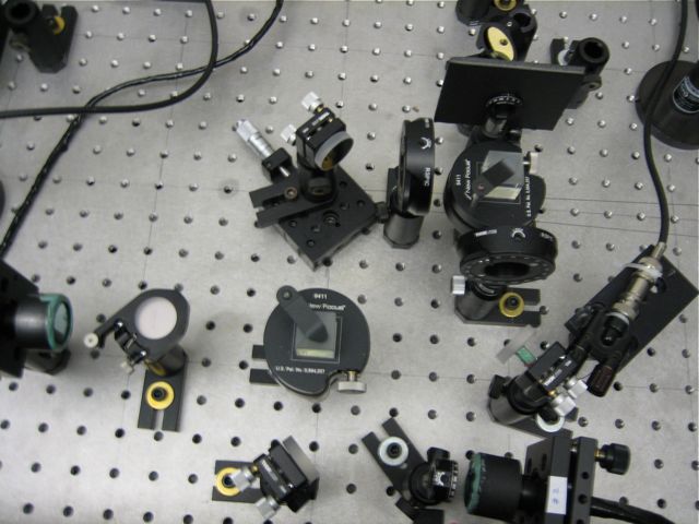
 Top view |
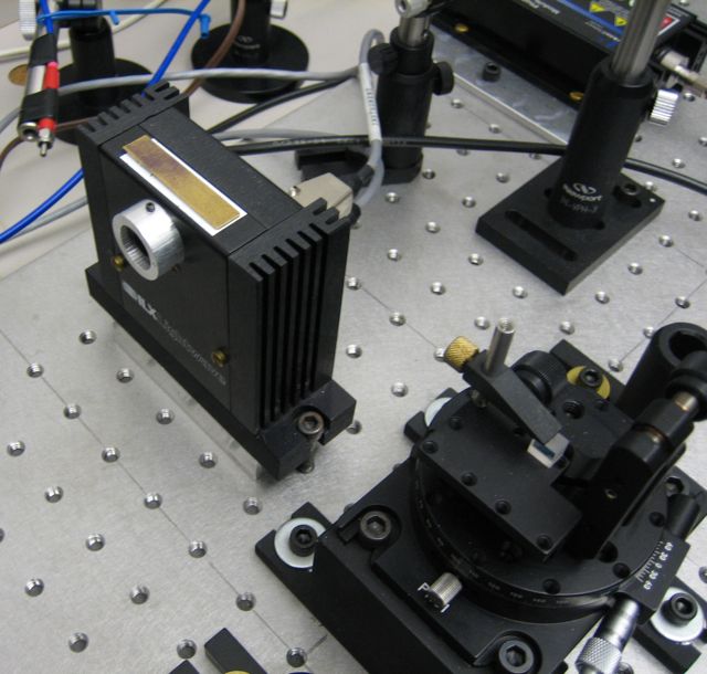
 BBO crystal mount |
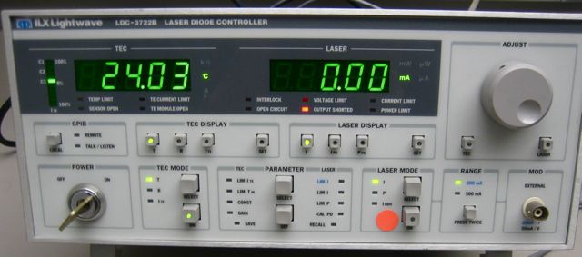 Laser controller |
Extensions
The following extensions are theoretically possible to do. I (Kai) tried to implement the HOM-interferometer - without succeeding. Though I would like to give you my alignment process and the problems I've come across.
Hang-Ou-Mandel Interferometer

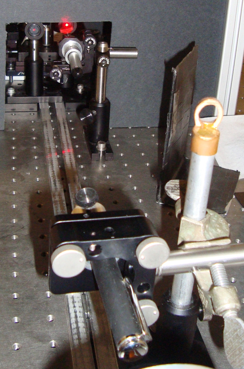
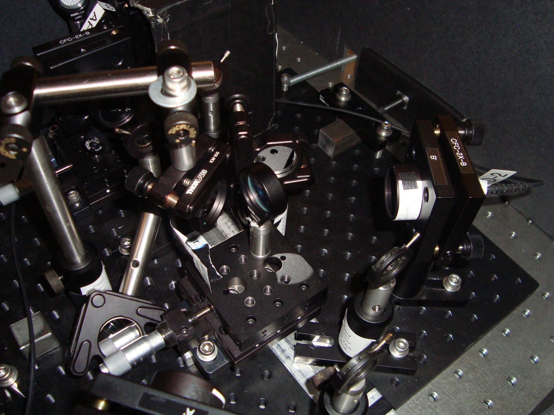
 Aligning the irises and the beam splitter plate |
 View from above |
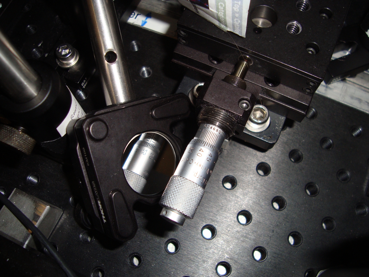 View of the reading of the micrometer of the beam splitter with the help of a mirror |
The theory of this experiment is described in the paper by Hang, Ou and Mandel [1].
- Start with arm A. The detectors A and B should still be in place from the earlier experiments which means that the maximum count rate is being observed at the current position and angle of A and B.
- Put the beam splitter (BS) in the exact place as seen in the picture. It is mounted on top of an aluminum bar. The micrometer of the BS should be at about 5 mm, when centered. (The violet laser beam should hit the BS in the middle of the it.) If this is not the case, move the arm A. If you didn't have to move the arm, continue with step 4.
- Change the position of detector A with the inchmeter and find the best position (highest incident rate of detector A). Adjust the angle as well while looking at the incident rate).
- Remember to write down all the measurements.
- Put in and align two irises; one in front of the detector and the other one at the edge of the black board. (See photo.) This will help you align two laser pointer. For this you need to use the red laser pointer and the optical cables. OR do the following step instead, though I find it not as accurate as the just described one.
- [Move arm A so the violet beam hits the center of detector A. (Do not change the position of the bar which is being pushed by the micrometer A, rather put a piece of aluminum in between the bar and the micrometer. Otherwise you will lose all your measurement results.) Put in and align two irises; one in front of the detector and the other one at the edge of the black board. (See photo.) This will help you align two laser pointer.]
- Repeat the last step (or step 5 respectively) with arm B.
- Mount the two red laser pointers and align them in accordance to the irises (see photo).
- Put the two mirrors and align both so the reflected and transmitted beams overlap each other and hit the same spot in the black side walls. The mirrors should be equidistant to BS. Put the detectors A' and B' into place where both beams overlap.
- Use the optical cables of detectors A' and B' and the red laser to align the angle of the detectors. The laser light should pass the irises and hit the center of the BBO mount.
Now you can turn on the laser diode and the APDs and check the incident and coincident rate in LabVIEW. The following filters can be mounted onto detectors A' and B':
- 810 nm interference filter with a 10 nm band width + 50 $\mu$m pinholes: I could hardly see any incidents. There were almost no coincidences A'B'.
- 810 nm interference filter with a 10 nm band width: Incident rates were at about 3000 1/s. The coincident rate was 1/10 of the one observed by HOM. I checked a displacement of about 0.6mm for the BS and the result can be found in measurements/20120919/HOM.xlsx. There is no pattern to be seen.
- long pass filters (FEL 800): The incident rates were for each detector at about 20,000 1/s. The coincidence rate was between 3 and 5 1/s. I checked the entire range of the BS and was not able to find the steep drop in coincident rates, though I did this rather quick and without making concrete measurements but by looking at the numbers on the computer screen.
So the major difficulty of this experiment is
- to align the mirrors and the detectors without seeing the 810 nm light and
- to find the correct position for the BS so both photons would have traveled the same distance when they interfere.
Mach-Zehnder Interferometer
This extension has not been tried to be implemented, yet. I find the set-up used by the University of Chicago very good. If this interferometer is to be used, it has to be set-up and aligned by someone knowledgeable. The process cannot be done by students in a few hours. So I recommend that this extension should only be set up permanently at some point.
References
- ↑ C. K. Hong, Z. Y. Ou and L. Mandel, "Measurement of subpicosecond time intervals between two photons by interference", Phys. Rev. Lett. 59, 2044–2046 (1987).
Useful References
- C.H. Holbrow, E. Galvez, and M.E. Parks "Photon quantum mechanics and beam splitters", Am. J. Phys. 70(3), 260-265 (2002)
- D. Dehlinger and M.W. Mitchell, "Entangled photon apparatus for the undergraduate laboratory" Am. J. Phys, 70(9),898-902 (2002).
- D. Dehlinger and M.W. Mitchell, "Entangled photons, nonlocality, and Bell inequalities in the undergraduate laboratory, Am. J. Phys. 70(9),903-910 (2002).
- E. J. Galvez, C. H. Holbrow, and M. J. Pysher, J. W. Martin, N. Courtemanche, L. Heilig, and J. Spencer, "Interference with correlated photons: Five quantum mechanics experiments for undergraduates", Am. J. Phys. 73,127-140 (2005).
- D. Branning, S. Bhandari, and M. Beck, "Low-cost coincidence-counting electronics for undergraduate quantum optics", Am. J. Phys. 77(7), 667-670 (2009).
- E.J. Galvez, “Undergraduate laboratories using correlated photons: experiments on the fundamentals of quantum physics,” in Invention and impact: Building excellence in undergraduate science, technology, engineering and mathematics (STEM) education, AAAS, pp 113-118 (2004).
- B.J. Pearson and D.P. Jackson, "A hands-on introduction to single photons and quantum mechanics for undergraduates," Am. J. Phys. 78(5), 471-484 (2010).