Design and Documentation (OTZ)
Contents |
Overview of Optical Trapping Lab
The idea of using light beams as tweezers to manipulate cells and tiny objects has been applied widely in physics and biology, including measuring forces generated by molecular motors and forces required to unzip DNA double helices. Optical forces generated by a laser beam focused through a high numerical aperture lens can apply pico-Newton forces and provide nanometer position resolution, providing a powerful tool for moving, controlling and measuring objects. In this lab, students learn the fundamentals of optical trapping, learn to calibrate an optical trap for position detection and force measurement using synthetic beads, and apply the technique to study internal transport by molecular motors in onion cells, flagellar locomotion in E. coli cells, and the stall force of a dynein motor molecule. The lab writeup is at Optical Trapping.
Acknowledgements
This experiment was developed under the direction of Professor Jan Liphardt. Suneet Upadhyay, an undergraduate Segre intern and student assistant, originally built the optical trap based on David Appleyard's design at MIT. Suneet wrote first version of the C#/.NET data acquisition and control application. Trevor Owen modified the apparatus and continued development of the software. Tom Colton further modified the apparatus after seeing improvements made by Steve Wasserman at MIT. In the summer of 2011, the trap was rebuilt to follow the MIT redesign by Bennett Sodergren and Tom Colton. Shawn Tang and Tom Colton improved the optics and started the dynein stall force experiment in 20011-2012. Harry Nunns worked out the protocol for the dynein experiment in the summer of 2012. The apparatus and initial staff time were funded by a generous gift from the Microsoft Research Division.
Apparatus
Our optical trap was inspired by one designed by Dave Appleyard at MIT, described on his web site and published in AJP[1]. He developed this for MIT's course Biological Engineering II: Instrumentation and Measurement. Appleyard's design had optical components in the beam path mounted on posts. We initially set out to replicate this, but found it challenging to align and were concerned about the hazard of an open beam. When Steve Wasserman took over MIT's instrumentation course, he redesigned the trap to mount all optics in a cage system with lens tubes shielding the beam whenever it is collimated. This version is easier to align and safer for students to use. We eventually rebuilt our trap according to his design. Thorlabs copied Steve's redesigned trap to sell in kit form in 2009. Thorlabs' design has gone through subsequent revisions and is used by both teaching and research labs. Nearly all of the kit components are from Thorlabs and include a higher quality motorized stage with feedback.
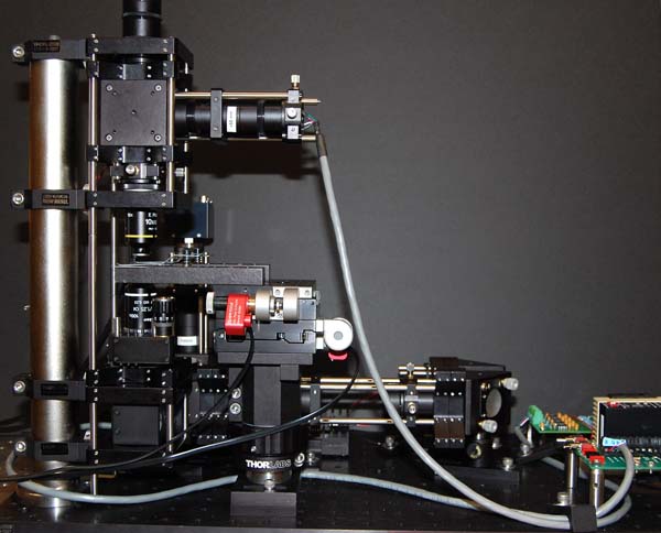
Current optical trap layout at Berkeley
We rebuilt our trap in 2011 according to Steve Wasserman's 2009 version in the MIT Biological Engineering lab course. We also added a fluorescence branch at that time to support a new experiment to measure stall forces of molecular motors.
For those who might want to replicate part or all of our apparatus, a parts listfor our trap is available. It details most of the optical components we use, but does not specify some important components, such as trapping laser, computer, DAQ card, optical bench, QPD amplifier, and illuminator power supply. A file of photos labeled with Thorlabs part numbers may be helpful in understanding how the apparatus is assembled. These photos show an optical trap in Steve Wasserman's lab at MIT that was assembled by Tom Colton in 2009. It does not include the fluorescence branch but otherwise is nearly identical to the current Berkeley trap.
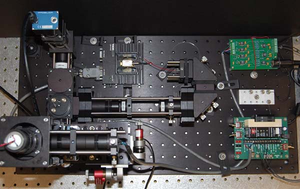 Top view |
Equipment Notes
Microscope illuminator: Blue LED (Luxeon LXK2-PB14-N00) attached to a heat sink.
Optical Table: Newport Vibration Isolation System Manual
DAQ breakout box: National Instruments BNC-2090A manual
Quadrant Photodiode: OSI Optoelectronics model SPOT-9DMI datasheet and mechanical specs. Also, see Application note "Non-Contact: Optical position sensing using Silicon Photodetectors".
Finnpipette Pipettors: Finnpipette Focus catalog.
Newport linear stages (2 used): Newport Model 423 datasheet, 2D views, 3D view.
Installing the Laser
Precautions: ALWAYS WEAR A GROUNDING BRACELET WHEN TOUCHING THE LASER OR ANY COMPONENT IN CONTACT WITH IT. Static discharge will destroy the laser. Also make sure not to kink or break the laser optic. If the fiber optic is bent more sharply then the minimum radius of curvature it will destroy it.
Due to the delicacy of the laser, it is advised that whenever dealing with a laser the user manuals for the TEC, LDC, Laser Mount and Laser all be read to make sure the functionality of each is understood well. These instructions are not complete, but give a general outline of how to proceeed.
Currently a LU0845 M200 Lumics laser (Data sheet for LU0845 M150) is mounted in a Thorlabs LM14 laser mount. The card in the laser mount is specific to the laser design. Most diode lasers use the same configuration, but the correct card is necessary as a wrong card will deliver voltages and currents incorrectly to the laser and likely destroy it. See also application note for similar Lumics laser modules. The thermoelectric temperature controller (TEC) is a Thorlabs TEC 2000 and controls the temperature of the laser diode to improve its stability. The laser diode controller (LDC) is the Thorlabs LDC 2000. The laser can be destroyed if too much power is provided. The laser mount allows the outputs on the TEC and LDC to be matched up to the correct pins on the butterfly laser diode. The laser diode has 14 pins which must each be driven correctly for the laser to function properly. The LDC and TEC are on long term loan from Jan Liphardt. He donated the current laser to the lab.
- First check to see how each pin in the 9 pin outputs of the LDC and TEC are driven. The manuals for the TEC and LDC each give a diagram of how each of the 9 pin outputs are driven.
- Check the laser manual to see which pin of the laser requires which input. The outputs of the LDC and TEC must drive the correct laser pin.
- The laser mount is the final piece of the puzzle, which must be configured to deliver the correct signal from the TEC and LDC to the correct laser pin. Check the laser mount to see if the 18 input pins (9 for each the TEC and LDC ) will correctly deliver power to the laser pins as specified by the laser manual and the TEC and LDC manuals. The manual for the mount may give incorrect pin assignments as the cards have been swapped out. To insure proper functionality, check which input corresponds to which contact by measuring the resistance between the contact and the input on the laser mount alone.
- If all pins are correctly assigned, the laser may be inserted into the mount according to operating procedures in the laser and mount manuals. WEAR A GROUNDING BRACELET!!! Insure during assembly that the laser fiber optic is not broken or kinked. This will cause backwards reflections into the laser which could destroy it. Make sure that nothing is bridging the gap between the two wires sticking up vertically from the laser mount, located behind the laser. This insures that the laser power cannot be delivered unless the TEC is on.
- Before attaching any components, the TEC and LDC controllers should be correctly set so as not to exceed any maximum laser power inputs. These can be set by consulting the Absolute Maximum Ratings in the laser manual and then correctly setting the TEC and LDC controllers to correspond to this. In addition, while setting these maximum ratings, the power input to the laser diode on the LDC should be set to zero, so that there is no sudden power surge delivered to the laser.
- Finally, once the TEC and LDC are set to driving the laser correctly, the laser is correctly mounted and its beam sent into a safe region, the TEC and LDC hooked into the laser mount, testing may begin.
Laser Beam Alignment and Collimation
If the beam is not centered and vertical within the microscope or does not fill the aperture of the objective lens, then the laser will fail to trap particles or trap them only against the slide. When the beam is properly aligned, a trapped particle may be moved vertically and horizontally without escaping the trap.
Safety Note: Alignment of the laser requires removing lens tubes that shield the beam, creating a potential exposure hazard to a 200 mW laser with an invisible beam. This work may be performed only by individuals who have completed the campus laser safety course and taken a baseline eye exam. Appropriate safety goggles must be worn during the alignment procedure.
Useful Tools
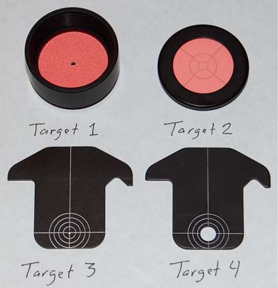
Useful alignment aids |
Targets that can be mounted on 1" ports or hung on cage bars to indicate the optical axis are indispensable. The targets pictured here are all available from Thorlabs. Target numbers indicated are referred to in the instructions below. In addition, a 6" lens tube and 1" irises that fit the lens tube are handy to have. A handheld IR video viewer is used to make the beam visible.
Procedure
A. Collimate laser
- To collimate laser, detach the laser terminator/collimating lens assembly from the cage by unscrewing it from the kinematic cage mount. Mount the laser and lens on a post on the table so that beam can be projected out the door and across the lab about 13 m (do outside of lab hours, block lab door for safety). Attach sheet of paper to a box to serve as target for laser. Start by collimating the beam within the experiment room with the door closed. A circular white target mounted on a post can be positioned at different distances on the table. Using the IR viewer, measure the diameter of the beam on the target at various distances with the aid of calipers. To focus the beam, rotate the plug holding the collimating lens with an adjustable spanner wrench (Thorlabs SPW801). When the beam is collimated, it should be approximately the same diameter at each distance, with some slight expansion of the spot but no waist. Open the door and measure the spot diameter across the room to get the best result. With laser power at 25%, the best that could be attained in August 2012 was a beam diameter expanding from 3.8 mm near the lens to just 8.4 mm across the room (13m).
B. Align laser with beam path cage
- Attach fiber terminator and collimating lens to kinematic cage mount, then all this to cage rods attached to steering mirror 1. Leave out the lens tubes here to make room to attach target 2 to steering mirror 1.
- Adjust kinematic mount to center the laser going into steering mirror 1. As an aid, hang target 3 from cage next to collimating lens.
C. Align beam through cube 1.
- Remove beam expander. Remove dichroic mirror in cube behind microscope and replace plug on left of that cube with target 2. Steering mirrors should start at neutral adjustment. Hang target 3 from rails where beam expander would be, close to steering mirror 2.
- To adjust beam in up/down direction, adjust upper knob of steering mirror 2 to get beam centered on the hole in the target placed by beam expander. Adjust lower knob of mirror 1 to move beam AWAY from center of target in turret. Repeat until beam is centered on both targets.
- To adjust beam in left/right direction (looking at targets), adjust lower knob of steering mirror 2 to get beam centered on the hole in first target. Adjust upper knob of mirror 1 to move beam AWAY from center of target in turret. Repeat. (Alignment of left-right/up-down can be done at same time.)
- Check to make sure there is no clipping of the beam when target 3 is removed from cage.
- Insert beam expander lenses and replace target 3 with target 4 (large hole). Bring beam back to center of target in cube by adjusting cage-mounted X-Y translator that holds the (-) beam expander lens.
D. Align beam through microscope
- Reinsert dichroic mirror in turret 1. Remove slide holder from stage to provide easier access and viewing. Remove objective and condenser lenses. Put target 1 with hole in place of objective. Put other target in place of illuminator (turret with dichroic above condenser can be removed, but it is possible to align with it in place as it transmits some IR).
- To adjust left to right (looking at targets): Move lower knob of steering mirror 2 to move beam AWAY from center of upper target. Turn the turret to bring beam back to center of hole in lower target. Repeat.
- To adjust front to back (looking at targets): Move upper knob of steering mirror 2 to move beam AWAY from center of upper target. Adjust middle set screw in turret top to bring beam back to center of hole in lower target. Repeat. (Notes: a. it is easier to center beam on lower target if you use target 2 in place of objective and sight down from directly above, b. do left-right and forward-back adjustments at same time.)
- Tighten the four nylon screws that attach turret to cube 1. To avoid rotating the turret during the tightening, tighten each screw only slightly each time, alternating screws across from each other followed by in sequence around the turret while pushing down on turret. Check the alignment again to be sure no movement occurred. Remove targets and insert objective and condenser. Re-attach lens tubes to enclose beam path. At this point, the critical part of alignment that determines trapping ability is completed.
E. Align Condenser and Detector Branch
- Remove dichroic mirror from the cube above the condenser (if you didn't earlier). Coarse focus condenser by shining on ceiling and adjusting condenser height to get even diameter beam all the way to ceiling.
- Center condenser by adjusting cage-mounted X-Y translator that holds condenser (with target 2 on top of turret).
- The geometry of the detector branch should provide for the back focal plane of the condenser to be imaged onto the QPD by a biconvex lens, as determined by the thin lens equation. A +35 mm or + 50 mm lens works well for this. [Nikon could not provide the location of the back focal plane of the 10x objective we use as a condenser, so we determined this empirically by shining a laser pointer through the lens and measuring its diameter at several distances. We concluded that the back focal plane is 7.05 mm inside the back of the lens, measured from the aluminum collar.] Using the condenser back focal plane as the object, $ \frac{1}{S_1} + \frac{1}{S_2}= \frac{1}{f}$ where $ S_1 = a+b $ in the diagram.


- Align beam to QPD. Remove target 2 from the cube and insert dichroic mirror turret. Remove QPD and in its place mount target 2 in a cage plate so target is approximately at same position as the QPD. Turn turret 2 to center beam vertically on target and tighten screws. Beam should be close to centered horizontally.
- Replace QPD. Fine adjustment of beam on QPD is routinely done during each experiment by adjustment of X-Z screws on cage plate holding QPD to zero the voltage recorded from the QPD.
F. Camera branch alignment
- When trapping, adjust camera steering mirror to get reflections of beam in center of field of view.
Measuring Laser Power
Meter: Thorlabs PM30 with S121B head, which is limited to 50 mW.
- Set meter to wavelength of trapping laser, currently 845 nm.
- With safety goggles on, laser interlock bypassed, and box open to allow access to beam path, place sensor head in beam path.
- Turn on laser, but limit power to stay within 50mW range of sensor.
- Use IR viewer to determine when beam is completely within the 9mm diameter sensitive area of the sensor.
- Power can be measured at several points along the beam path, but the one that counts is what goes into the back of the objective. To measure this, remove objective lens from its holder and center sensor over the hole.
When measured on March 10, 2011, the following data were obtained:
With laser controller set at P = 0.400,
Pmeas = 45.0 mW just before 1st steering mirror (after beam expander)
Pmeas = 42.1 mW just before dichroic mirror
Pmeas = 41.7 mW just after dichroic mirror
Pmeas = 35.0 mW just before objective lens.
With laser controller set at P = 0.500,
Pmeas = 44.3 mW just before objective lens.
Highest power setting of laser controller is P = 1.05, which should correspond to a power measured at the objective of 93.0 mW assuming laser power increases linearly with the power displayed by the laser controller.
The calculated highest power we are getting just before the 1st steering mirror is 118 mW, which is about 79% of the rated power (150 mW) of the laser. This is after losses to the fiber, collimating lens, and beam expander.
The biggest drop in the beam path is between the dichroic and the objective. This 16% drop occurs in one component, the 45 degree mirror below the microscope. This mirror is outside the box and faces upward, so has accumulated a lot of dust and may have oxidized. Replacing this mirror and protecting it from dust would be desirable.
Fluorescence
To add fluorescence to the optical trap, we will use Cy3 as our fluorescence dye.
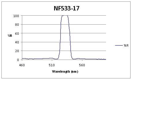
Figure 1. NF533-17 reflection spectrum at normal incidence.
It has an excitation wavelength of ~554nm and an emission wavelength of ~570nm. To use the fluorescence laser, IR laser, and blue LED illuminator (~460nm) without needing to switch the lens, a notch filter is required. The notch filter available from Thorlabs (NF533-17) has a center wavelength at 535nm and would reflect at 535nm but transmit light to either side of this peak. The reflection coefficient at this wavelength is 99.70942, which was measured at normal incidence. For our optical trap, the light would be incident at 45 degrees, which causes the reflection spectrum (figure 1) to shift to the right according to the equation $\frac{\lambda_\phi}{\lambda_0}=\frac{\sqrt{N^2-sin^2\phi}}{N}$ where
$\phi =$ angle of incidence
$\lambda_0 = $principle wavelength at $0^o$ angle of incidence
$N =$ index of refraction
$\lambda_\phi =$ wavelength at $\phi$
For the index of refraction, 2.1 was used at the recommendation of Thorlabs. This may or may not be accurate because the coating on the notch filter was provided to Thorlabs by a different company, and Thorlabs does not have an exact value. N=2.1 is the index of refraction of most of their other filters (other than notch filters), so they suggested it for the calculation. Using the above equation, in order for the center wavelength to be at 535nm with an incident angle of 45 degrees, the center wavelength would be 568nm at 0 degrees incidence. However, Thorlabs does not have a notch filter with these specifications. Another company, Chroma, does not have notch filters, so another option is to use a simple band pass filter. This means that to use fluorescence, multiple filters will be required and will need to be switched while using the trap.
Software
We currently use a Matlab program to acquire and process data from the QPD and to control the stage picomotors. This program was modified from a program used at MIT for their traps, which now use all Thorlabs components, including the stage, laser driver, and QPD amplifier.
We originally used a program written here in C# and .NET to control the stage and camera, to analyze particle tracks from the camera images, and to take and process voltage data from the QPD. The program is available for download as OpticalTrap1.0 Zip file.
Flowchart for old C#/.NET software
In this series of experiments, students use an optical trap to calibrate an optical trap for position detection and force measurement using synthetic beads and apply the technique to study bacterial motility. The software must position the stage, and measure the displacement of objects on the stage.

Flow Chart for Optical Trap Software
Modules
- Experiment Module, User Input
- This module will set up the different experiments.
- It must allow the user to position the stage and use the camera to observe the slide, in preparation of starting a calibration sequence or performing a measurement.
- Stage Positioning & Dead Reckoning
- This module controls the picomotors (stepper motors) by connecting to a DAC motor interface.
- It must be able to keep track of the stage position relative to a user defined reference point.
- Particle Position Readout
- This module must accept calibration data (from a file or memory) and then readout the photodiode signal as a position vector.
- Particle Imaging
- This module images the slide and presents a real-time readout to the user. It may optionally include visual tracking of slide objects.
- Data Logging
- The results of an experiment run are collected and analyzed, for example by plotting the extension of the DNA tether vs. the applied force (proportional to displacement).
Sections removed from lab writeup
Power Spectral Density (PSD) Peak Value Method
This procedure requires a floating bead in deionized water. Though this calibration lacks accuracy, it is very fast and easy. It cannot be used as the sole source for the sensitivity of the trap. For this procedure, you will need to trap a bead in the laser. Once this is done, you can simply read off the Peak Value, $P^v$, of the Power Spectral Density * frequency squared (PSD*f^2) graph. This is the height of the graph at the plateau of the PSD*f^2 graph. This can be used to find a rough estimate for the voltage to displacement calibration using the equation for the sensitivity in [Volts/meter]: $ \rho = \left(\frac{P^vd}{5.0*10^{-20} m^3/s}\right)^{1/2} $ Where $P^v$ is the peak value. This assumes the fluid is water.
Stoke's Drag Method
This method uses the force created by a laminar flow of fluid past a spherical bead, given as: $F = \beta v $, where $\beta = 3 \pi \eta d$ as given above, and v is the velocity of the water. This is used to estimate the restoring force of the trap. The idea is to induce a constant laminar flow, and by estimating the velocity of the flow when the force of the water is in equilibrium with that of the trap, predict the force on the bead.
 |
One way to create a laminar flow is by making a flow cell. This can be done by using about 3 layers of double sided tape on either side of a microscope slide and a coverslip on top to create a small rectangular flow cell, as in the picture. The coverslip in the picture, show in grey, is much larger than the coverslip provided. Set up this flow cell, fill with a 1:500 part 2 micron bead to water solution and place on the stage with the coverslip down. Using the Prosilica Viewer, the beads can be seen in suspension. Using an approximately 1x2" piece of Kimwipe, a corner can be rolled into a small point. Care must be taken to make several of these points the same. The thickness of the tip and the areas near the tip are the most critical in determining flow rate. Some will be used to estimate the flow velocity of the water, while other similar ones will be used to induce this flow once a bead is trapped. Th point of the Kimwipe can then be touched to the edge of the water solution in the flow cell to induce a laminar flow of the beads near the center of the flow cell. Near the edges of the flow cell, the viscosity of the water will change the flow. The velocity must be estimated from the rate the beads move at, once a steady flow has been established. There should be a brief acceleration of the beads before an approximately steady flow rate is established. Due to the rapid rate of flow of the beads, it will be necessary for one person to start the flow of solution and another to watch the viewing screen and estimate how long it takes for a bead to go across one entire screen. This can be done with a stop watch. The full viewing screen is 659 x 493 pixels. This can be converted to about 44.5 x 33.3 micrometers using the pixel to distance conversion. After every trial of sucking up water using capillary action of the Kimwipe, more solution must be added to the flow cell to maintain the same initial set up. Once the velocity of the flow near the center of the cell has been established, a bead can be trapped near the glass and moved to the center of the trap. Using the QPD position readout GUI, an 8 second, 1kHz sample can be taken of the bead while a laminar flow is induced around it. This data should show a part where the bead is trapped and in constrained brownian motion and another part where the bead has been shifted to the side, due to the force of the water flow. If a constant laminar flow is established, the two forces will be at equilibrium for some period, which should show up in the positional data. The average deviation from the center of the trap due to laminar flow can then be estimated using a graphing program like Excel. This will give an average deviation, <x> and knowing the force on the bead induced by the flow of water past it, one can estimate the trap stiffness, k. Due to the difficulty in inducing a laminar flow using the Kimwipe, it is suggested that the team take several data sets (atleast 5), each time refilling the flow cell to restore original conditions.
 |
At right is an example of a data set of 8 seconds, sampled at 1 kHz, where laminar flow was induced using the flow cell. It can be seen that the flow becomes approximately steady between 2 and 4.7 seconds in the Y direction. Here the force of the trap and the laminar flow force came into equilibrium. The bead remained in this position, vibrating around this point due to the normal Brownian motion. After that, the Kimwipe was removed and the bead returned to normal Brownian motion centered in the trap.
This method is not to be used alone because the difficulty of the set up can cause large errors. It does, however, have the advantage of using a completely different set of physical data to estimate the trap stiffness than the previous two estimations. It should also be noted that the water will flow differently if near any edge of the flow cell due to interactions of the water with the edges. The solution can be modelled as an incompressible Newtonian fluid just as water. A discussion on sources of error, assumptions and the physics used to estimate the flow of water is necessary here.
Another way to see the drag effect on the bead, is to first trap a bead in a dilute (1:3000 or so) solution prepared in the normal "well" fashion and move it away from the cover slip. Then with some practice, you can learn to turn the knob with a regular speed. Estimate the rate you are turning the knob using stuck beads and a stop watch. If you start an 8 second 1 kHz reading and began the movement slightly after starting, the program will graph the positional data from the QPD. If a smooth turn can be accomplished, you should see data similar to that of the flow cell shown above. I found it hard to avoid accelerating the knob rotation speed because the static friction presents a significant barrier at the beginning of the rotation. For this reason, the data is often irregular. However, this is a fast and easy way to see the effect, though useful data is hard to obtain from this method.
An important question to ask is: Could the stepper motor be used create a laminar flow of water past the bead? Why or why not?
References
- ↑ D.C. Appleyard, K.Y. Vandermeulen, H. Lee, and M.J. Lang, "Optical trapping for undergraduates." Am. J. Physics, 75(1) 5-14, (2007) Design, construction, and use of optical trap for a course in MIT's Biological Engineering Department.