BMC - Experimental Procedures
All pages in this lab
II. Simulating Brownian Motion
III. Experimental Procedures
IV. BMC Software
Contents |
Microscope How-To

The BMC Station |
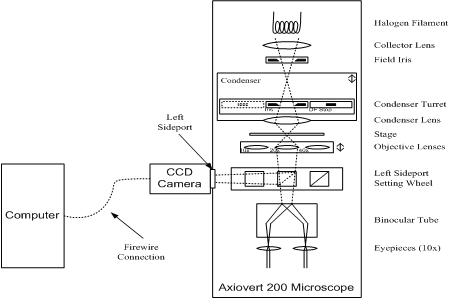
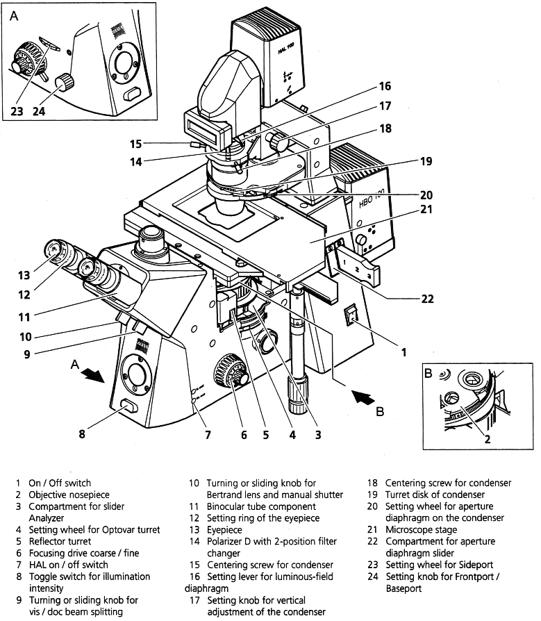
Block Diagram |
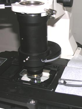
You will use the Zeiss Axiovert 200 inverted compound microscope illustrated above. Starting from the top right of the diagram, the microscope has a variable intensity halogen light source. A condenser focuses light from the halogen bulb onto the sample under observation. A rotating turret in the condenser holds several irises and stops that are used for different contrast methods such as bright- and dark-field. (As shown, the condenser iris is selected, as would be the case for normal bright-field illumination.)
The objective nosepiece rotates to select one of four objective lenses: 5x, 10x, 20x, and 40x. Although they are depicted as simple lenses in the diagram, the objectives are actually sophisticated, compound optical elements. More information about objectives can be found in references 6 and 7. Specifications of the objectives may be found at the Zeiss website.
Light enters the microscope body through the selected objective and is optionally split into two paths. A setting wheel selects whether 0, 50, or 100 percent of the light is diverted to the left sideport for the camera. The remaining light goes on toward the eyepieces. A CCD camera is mounted with its sensor at the focal plane located just outside the sideport. Images captured by the camera are transferred to the PC via a Firewire connection.
A binocular tube splits the image headed toward the eyepieces in two for direct observation with both eyes. The eyepieces are 10x, providing overall magnification of 50x, 100x, 200x, or 400x depending on which objective is selected.
Look over the detailed schematic of the Axiovert 200 microscope. You will notice some differences between the microscope in the drawing and the one in the lab – most significantly in the condenser (described below). To become familiar with the microscope controls, follow the instructions below to make a slide with a combination of 10µm and 0.44µm polystyrene spheres and then view it in both transmitted light and dark-field illumination. But first some general warnings:
* The microscope is a delicate instrument. It is never necessary to force any adjustment.
* Do not remove any parts from the microscope (except for eyepieces) or attempt to clean the optics.
* If the microscope needs cleaning, ask a GSI or Don for help.
* Do not use canned air on the microscope. It can leave a difficult-to-remove residue.
* To lengthen the lifetime of the halogen lamp, turn off the light source with the HAL on/off switch (Schematic-7)
  when it is not in use.
How to pipet
The pipettes are located against the wall in a special holder (suspended above the shelf, about eye level)
Forward Technique: Fill a clean reagent reservoir with the liquid to be dispensed.
- Depress the push button to the first stop.
- Dip the tip under the surface of the liquid in the reservoir to a depth of about 1 cm and slowly release the push button. Withdraw the tip from the liquid touching it against the edge of the reservoir to remove excess liquid.
- Deliver the liquid by gently depressing the push button to the first stop. After waiting about one second to fully empty the pipette tip, continue to depress the push button all the way to the second stop. This action will empty any remaining liquid.
- Release the push button to the ready position.
If necessary, change the tip and continue pipetting.
-
- Adjust the volume of fluid dispensed by rotating the thumbwheel until the desired volume
Never allow liquid to enter the body of the micropipette
-
- To avoid contaminating the nanoparticle suspensions, wear gloves and put a fresh filter tip on the pipette each time you dip it in a new solution.
- Shake stock suspension bottle to separate and mix particles.
Make a viscous suspension
A solution will consist of three parts, water, which makes up most of the solution, a solute (either PVP or glycerol) to provide the viscosity, and the beads which we will then observe.
Water can be located in the large squeeze bottle marked "Deionized Water," be sure to use this rather than tap water as tap water will fill your slide with various unwanted particulate matter.
The Solutes can be found in the upper cabinet and are also clearly marked. Use the long and thin metal scoops/spatulas to measure out the PVP and the large-volume pipette to measure out the glycerol. Note that the glycerol is extremely sticky (ie viscous) and will not be measured precisely using the pipette as it will stick to both the inside and outside of the filter tip. To measure both the PVP and glycerol it is best to use the scale located at the lab station.
Computing viscosity
Use this table to compute the required dilution of the solvent. The PVP in the lab is in pure powder form. The stock Glycerol is a thick liquid with >99% purity. It will require some care to measure the pure glycerol accurately, since it tends to stick to the sides of the pipette tip. For this reason, weighing the glycerol before adding the water is probably a better technique than adding the glycerol to the water.
PVP and Glycerol Viscosity versus Concentration

Viscosity (cP)		PVP to Water Ratio (by weight)	       Glycerol to Water Ratio (by weight)
1.66		        0.50% : 99.5%                 	       18.0% : 82.0%
2.50		        1.00% : 99.0%	         	       32.2% : 67.8%
4.65		        2.00% : 98.0%	           	       44.2% : 55.8%
13.2		        4.00% : 96.0%		               64.5% : 35.5%
You may either use these values or interpolate between them (are the relationships linear?).
- Take out a new plastic vial to contain the viscous solution
- Turn on the balance by pressing the button labeled with a one inscribed in a circle
- Place vial on balance and ensure all of the doors on the enclosure are shut.
- Zero/Tare the balance by pressing the 0/T button to cancel out the weight of the vial
- Place a moderate amount of solute (either PVP or Glycerol) into vial
- Weigh the amount of solute using the balance
- Calculate how much water is needed to obtain the desired viscosity using the table above
- Add the appropriate amount of water to the vial
- This can be done either by measuring the volume with the pipette or by squirting water into the vial using the squeeze bottle and measuring the amount using the balance.
- If you use the pipette to transfer deionized water you may find it easier to squeeze a large amount of water into a glass beaker and then use that as your reservoir
Creating Polystyrene Suspensions
Beads are located (and should be kept) in the refrigerator. Each of the vials is clearly marked with the size of bead that it contains. (Note: The sizes reported on the vials are mean particle diameter, not radius.) These vials are often extremely concentrated and you may wish to create your own diluted solution to work with.
Note that the densities vary to a small extent between the different size particles. For this reason, the following procedure may need to be adjusted slightly for each of the different particle sizes.
- Remove a bead vial of the desired size from refrigerator
- Using a NEW filter tip extract 10μL from the vial and deposit into a new plastic vial
- Use the large volume micropipette to add 100μL of desired viscous solution to the same plastic vial
- Cap vial using a plastic vial top and shake it vigorously to ensure it is mixed uniformly.
- Next, extract 10μL of the newly created suspension from the plastic vial and deposit it into a new plastic vial (Vial 2).
- Add 500μL of the same viscous solution to Vial 2.
- Cap vial using a plastic vial top and shake it vigorously to ensure it is mixed uniformly.
Repeat this process with each experimental condition selected.
Make a slide
Now that we have a proper vial of viscous bead solution made up we need to transfer a sample of it onto a slide so that we can observe the beads' behavior.
- Take out a slide from its box and carefully rest in a position to minimize dust contamination.
- Place a self-adhesive reinforcement ring onto the center of a new slide. This will create a well for the solution and keep it from drying out.
- Make sure that this label is well pressed down onto the slide to ensure that liquid isn't sucked out towards the open air. Rubbing the edge of another slide over the coverslip provides a good method of pushing down the well without contaminating the slide with oils from your hands.
- Use the pipette to transfer roughly 10μL of your bead solution into the center of the well
- Cover the slide with one of the small 18x18mm coverslips
- It is important to ensure that air bubbles do not form beneath the coverslip.
- To prevent this, rest one edge of the coverslip on the slide and then let the other side drop onto the slide. (Capillary action will adhere the coverslip to the slide.)
- Move the objective lens away from the microscope stage first before placing the slide onto the stage.
- The entire carrier arm that holds the HAL 100 illuminator and the condenser tilts backward on a hinge to facilitate access to the microscope stage. Push back gently on the angled metal nosepiece just above the LCD display until the arm comes to a rest (Figures).
- Our microscope is an inverted microscope and as such the sample (ie, side with the coverslip) should be positioned such that the coverslip is on the bottom side of the slide (So the upside-down orientation compared to how you prepare your slide). This will ensure that the sample is closest to the objective. You will not be able to focus on the sample using the 40x objective if this is not the case.
Microscope Figures
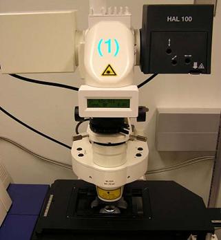
Place hand on position number (1) then gently tilt back top of microscope |
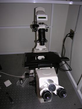
Putting a Slide on the Microscope Stage |
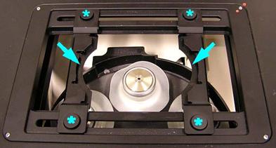
Place microscope slide between the arrows shown above |
Slide installed onto microscope stage |
Schematic of Axiovert 200 Microscope
View the slide in transmitted light
Microscope images look best when properly illuminated. The procedure developed by August Köhler’s is nearly universally used to achieve uniform illumination with little reflection or glare and minimal sample heating. In this step, you will view your sample under Köhler illumination.
As shown in Figure 4, there are two irises in the illumination path of the microscope. The one on top (closest to the light source) is called the field iris. The condenser iris is a little farther down. The adjustments for both irises are highlighted in Figure 2. The condenser iris adjustment is located at the edge of the turret disk near the bottom of the condenser. You will adjust both of these irises to achieve the best image.
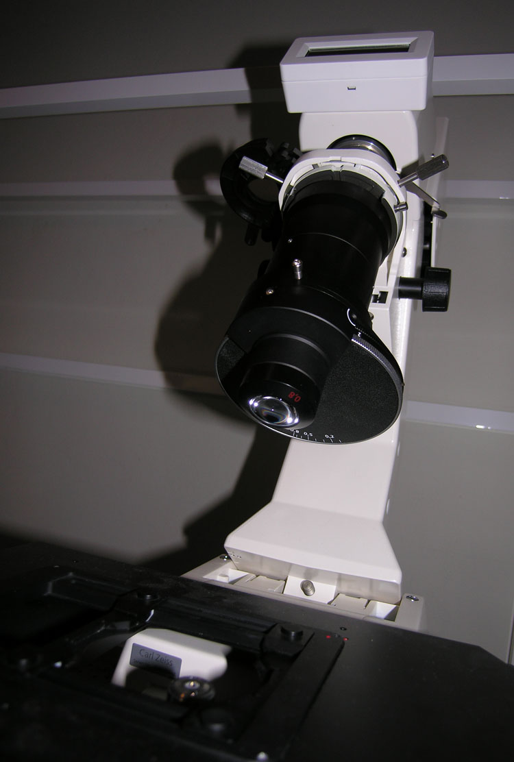
Figure 4: Picture of Field Iris, Condenser Turret, and Condenser Iris Adjustment
Fig. 2 is a picture of the actual condenser assembly you will find in the lab. The markings on this condenser are a bit confusing since it was designed to be used mainly in upright microscopes instead of inverted models such as the Axiovert 200.
It is necessary to go through this adjustment procedure every time you change objectives or samples.
- Use the On / Off Switch (Schematic-1) to turn the microscope on. Rotate the turret disk Schematic-19 on the condenser to the transmitted light position. (See Fig. 4 for a picture of the actual turret disk.)
- You will see an upside down number "2" just to the left of the condenser shaft when you have the correct setting. Tilt the condenser back and hold a piece of paper under the bottommost lens. If the spot gets brighter and darker as you rotate the field iris ring, you have the right setting.
- Rotate the side port setting wheel (Schematic-23) to the 100% visual setting (looks like two concentric circles). You can also set it to 50/50 visual/Camera or 100% camera.
- Open the condenser iris all the way using the Setting Wheel for Aperture Diaphragm on the Condenser Schematic-20. This is a thin, silver wheel on the turret.
- Select the 10x objective by rotating the objective nosepiece (Schematic-2) until the display reads 10x. Physically look at the body of the objective to make sure it is on the correct setting (10x should be setting #2).
* It is possible to make the tip of the objective collide with the slide.
* If you crash an objective into the slide, you will very likely break the slide.
This will release the liquid from the slide on to the objective and make it very dirty.
Try very hard not to do this.
- You must set up Köhler illumination each time you change objectives.
- Focus on the sample using the coarse and fine focusing knobs (Schematic-6).
* When you get close to the proper focus, it is an excellent idea to engage the focus limiter
at a setting slightly higher to reduce the chance of running in to a slide.
* Avoid focusing on slower particles because they are close to the edges.
Adjusting the field and condenser irises
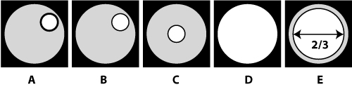
Fig. 5. Adjusting the irises
Do not skip this step. The microscope must be focused on a sample to properly set up Köhler illumination.
- Adjust the distance between the eyepieces on the binocular tube by rotating them toward or away from each other. When the distance between the eyepieces matches the distance between your pupils, you will see images in both eyes. You can make both eyepieces higher or lower by arranging them in a right-side-up or inverted V configuration. There is a scale on the binocular tube that will allow you to easily reestablish the correct setting if it has been changed.
- The samples in this lab are difficult to focus on because they have very little contrast. If you have trouble focusing, try starting with the 10x objective. At higher magnification, it is sometimes helpful to focus on the edge of the slide first to get the setting close.
- The eyepieces are designed to be used while wearing eyeglasses. If you do not wear glasses, don’t get too close to them.
- Close the field iris (Schematic-16) until you can see its outline in the eyepieces (Fig. 5a). If you do not see the outline in the eyepieces, the condenser may be too high. Move it down using the height adjustment knob (Fig. 5b). Make sure not to lower the condenser into the slide.
- Bring the field iris into focus by moving the condenser up or down using the condenser height adjustment knob (Fig. 5b). Do not adjust the focus of the objective. When you have successfully focused the condenser, you will see a regular hexagon of light through the eyepieces. Continue to focus until the perimeter of the hexagon is highly defined.
- Remove one eyepiece. Center the image of the iris using the condenser centering knobs (Schematic-18) until the image looks like Fig. 5c.
- If you do not see any light, open the field iris until you can see its edge. Use the condenser centering knobs to move the opening closer to center and then continue closing the field iris.
- Replace the eyepiece and look at the position of the hexagon. Use the condenser centering knobs (Schematic-18) to further center it within the field of view.
- Looking into the eyepieces, open the field iris until its edges are just out of view (Fig. 5d).
- Use the image intensity switch on the front of the microscope to set a comfortable overall illumination level.
- Never use the field or condenser iris to adjust the brightness.
- Change the focus to see a very little portion of the particles for a movie. After you change the focus, let it stand. Have about 1-5 particles in view.
- Look at the 10μm spheres with the 20x and 40x objectives. You may have to refine the focus as you increase magnification. Remember to set up Köhler illumination each time you change objectives.
Why do the PS spheres appear bright in the middle?
Set-up darkfield illumination
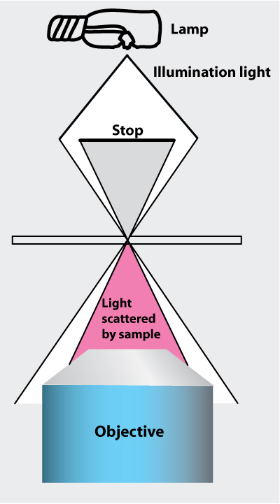
Fig. 6. Principle of dark-field illumination. all the illuminating light is rejected, and light scattered by the sample is collected by the objective |
Dark field illumination allows for observation of small particles under the microscope that would not normally be visible. This is due to the scattering of light onto the particles. The effect is similar to looking at stars during the daytime versus night.
- Select the 20x objective and establish Köhler illumination.
- Rotate the condenser turret disk (Schematic-19) one position to the right. You should see an upside down number "2" just to the right of the condenser column.
- Remember that for bright field, the upside down number "2" is to the left of the condenser column; the upside down number "2" is to the right of the condenser column in dark field.
- To get an idea of how this affects sample illumination, tilt the condenser column back and hold a piece of white paper under the condenser. You should see a disk of light. In this position, an opaque disk blocks the light in the middle of the illumination field.
- Open the field iris all the way
- Increase the light intensity using the Toggle Switch for Illumination Intensity (Schematic-8). You will need to turn the light level up significantly in order to see the small amount of light scattered by the smaller nanoparticles (even though the PS spheres will be easily visible). Increase the illumination until you hear a beep, and the level will be approximately correct. (The beep indicates that the halogen light source is set to the correct level for color photography, incidentally). Note: One beep indicates set point, three beeps indicate maximum light.
- Adjust the condenser slightly up or down to obtain an even, dark background. If you properly set Köhler illumination, the required adjustment should be very small.
- You should see something similar to Fig. 7.
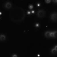
Figure 7: Darkfield image of single 100 nm diameter gold nanoparticles
Viewing / Tracking Particles in Viscous Suspensions
Now that suspensions have been made for each experimental condition, and the microscope has been fully configured, we are now ready to take data.
Estimating the Pixel to micron conversion factor
Prepare a solution of 10 µm PS beads in the same manner as the viscous suspensions were prepared, except use deionized water instead of viscous solution.
- Make a slide, and place it into the microscope.
- Move the Sideport Setting Wheel (Schematic-23) to the 100 Percent setting.
- Move the stage around until a number of particles can be viewed in the eyepiece.
- Change the Sideport Setting Wheel to the setting that diverts 100 percent of the light to the camera (it looks like an arrow pointing towards the computer)
- Open the Brownian Motion application and press Camera Go on the Control window.
- Note: to close ALL program windows click the X at the top of the window on the camera window.
- Adjust the microscope so that the particles are clearly visible on the computer screen (the camera requires more light than is necessary when viewing through the eyepiece).
- You can compare the image on the computer with that through the eyepieces using the 50 percent setting on the Sideport Setting Wheel.
- Use the resizable box in the software to inscribe one of the spheres. The size of the box is written to the bottom of the Control Window whenever it is changed. To re-size the box, hold down either Shift or Ctrl while clicking the side of the box.
- Record the number of pixels the sphere takes up on the screen
- Repeat this measurement a number of times to obtain a statistically accurate number.
You should obtain values of around 0.3-0.5 µm/pixel for the 20x objective. You will use your value as the conversion factor in the software.
Obtaining Data from viscous solutions
- Place a slide with one of the selected experimental conditions into the microscope.
- Move the Sideport Setting Wheel (Schematic-23) to the 100 Percent setting.
- Move the stage around until a number of particles can be viewed in the eyepiece.
- Change the Sideport Setting Wheel to the setting that diverts 100 percent of the light to the camera (it looks like an arrow pointing towards the computer)
- Open the Brownian Motion application and press Camera Go on the Control window.
- Adjust the microscope so that the particles are clearly visible on the computer screen (the camera requires more light than is necessary when viewing through the eyepiece).
- You can compare the image on the computer with that through the eyepieces using the 50 percent setting on the Sideport Setting Wheel.
- Track several particles and obtain the diffusion coefficients.
- Enter all of the information into the control window
- Enter the minimum particle size (in pixels)
- Enter the maximum particle size (in pixels)
- Enter tracking reach (in micrometers)
- Enter the Pixel to Meter conversion (this is the µm/pixel value from above)
- Enter a desired filename (default is particles.txt)
- Be sure it ends in the extension .txt
- Change the filename each time you take data or it WILL be overwritten
- Select Find Particles
- Adjust the ZScore Threshold as necessary
- Select Track Particles
- When you are ready to take data, press the Set Start Time button.
- When you are done tracking, press Compute Diffusion Coefficient or Save Particle Data (which ever you wish to do) -- Note you can calculate the diffusion coefficient manually when you save data. 15 seconds is sufficient to obtain reasonable data.
- Enter all of the information into the control window
Repeat this for each experimental condition selected.
Note: Watch out for bulk flow. If you see a number of particles moving in one direction, they are likely undergoing bulk flow. This could be due to evaporation of liquid from beneath the coverslip or an air bubble popping, or various other conditions. If you see bulk flow occurring, your data will be skewed. Make sure there is no bulk flow when collecting data.
This should conclude Part I of the experiment
Tracking Particles in a Living Cell
Making an onion slide
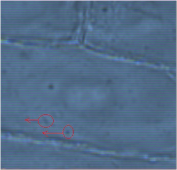
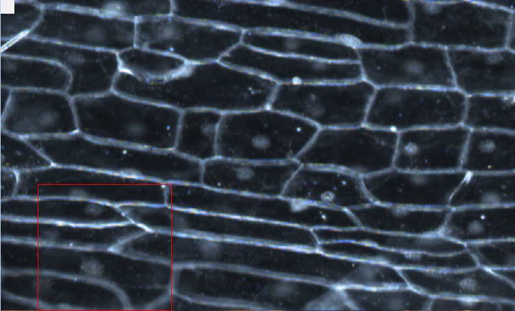
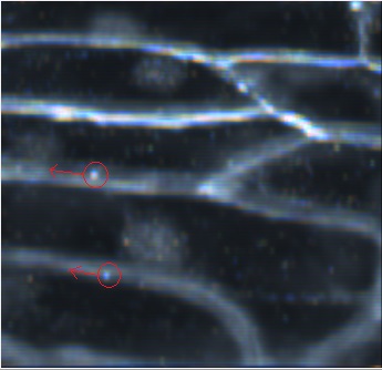
Objective 3 (40X magnification) image of an onion cell. The red square is enlarged in the next picture. The onion's cells possess an interesting property which is that the particles tend to use the cell walls like highways, and tend to travel along these walls (although they will not solely be traveling down the cell walls Objective 2 dark-field image of the onion cell. The intracellular particles are now white dots |
Bright-field image magnified image. The red circles with arrows indicate the particles that are traveling down the cell wall
Dark-field zoomed-in image of the onion cell. The red circles with arrows indicate the particles (now appearing as bright white dots) that are traveling down the cell wall. |
- Before coming to lab obtain an onion from your favorite produce store. If you have forgotten one, you can try the Seven Palms deli located conveniently at Euclid and Ridge, perhaps a five minute walk from LeConte.
- Use a knife, box-cutter, razorblade or whatever other cutting tool is provided to cut out a one inch cube from the onion AT ITS DEEPEST LAYER.
- Take one of the lower layers (activity depends somewhat on depth) and remove the lower membrane using the forceps. This is similar to pulling off a sticker.
- The membrane is a single layer of cells, which makes it particularly clean when viewing through a microscope. It should appear translucent and should be relatively strong.
- Make a slide using this membrane
- Place a drop of saline solution onto a clean slide (don't use water)
- Place the membrane onto the slide
- Drop a couple more drops onto the onion and cover with a large 24x60mm cover slip
- Blot excess liquid using a paper towel
- Mount onto microscope
- Keep in mind that the lifetime of an onion slide is about 30 minutes before it dries out.
- Put the remainder part of the onion into a plastic baggy and put it into the refrigerator.
- For the benefit of all future users of the refrigerator, please remove your onion when you have finished the lab. Do not leave it for the next group.
- Note: It's not uncommon for some onions to not have much activity. Some students have had success bringing a few different types of onions and searching for the highest activity levels. You should be able to see hundreds, if not thousands, of tiny bodies in motion.
Making Observations
First you should spend a little while looking around, trying to find some regions of interest. Start with bright-field illumination (Objective 3, upside-down 2 to the left of the condenser). Adjust the brightness of the lamp as needed, along with the focus. Note the different types of movement and where they tend to occur. In particular, be sure to investigate regions around the cell walls, regions around the nucleus, and also see if you can find anything happening within the otherwise empty center of the cell. Most of the activity happens on the lower and upper layers of the cell as the center is occupied with the vacuole which should be devoid of anything except water. If you scan through the depths of a few cells carefully however (using the focus knob to move in depth) you should be able to find isolated actin fibers which make for very clean data-taking. Next, try dark-field illumination (Objective 2), and compare your camera images to the pictures above for both illumination regimes. Remember that each time you change the objective (and slide, for that matter), you must refocus the objective using the large knobs on the side.
Your data analysis will be much easier if you can isolate the forms of movement within the cell and only take data on one type at a time. Otherwise you may have to manually sort through particle trajectories.
Take data using the particle tracking software (Brownian Motion Application) as you did with the viscous suspensions.
- Locate a particle that does not appear to be moving around very much (i.e. look for a particle undergoing Brownian motion rather than active transport)
- Determining the diffusion coefficient of the particle.
- Do this several times to obtain a statistically acceptable number.
- Track a number of particles undergoing active transport within the actin filaments
- Repeat this for a number of different cells.
- Change the microscope to obtain a transmitted light image of the onion cells
- Determine the size of the particles by counting the number of pixels each one take up on the screen as you did with the ten micron polystyrene spheres to obtain the pixel to meter conversion
- Repeat this step as necessary to obtain a statistically acceptable number.
This should conclude Part II of the experiment