NLD - Experiment and Procedure
Pages of this lab.
I. Non-Linear Dynamics and Chaos
II. Experiment and Procedure
III. The custom VI's for this experiment & Appendix
Contents |
The Experiment Apparatus
This experiment uses an Intel CPU based computer, running the Windows operating system. The main tools are a data-acquisition computer-interface card and the LabView software package. The data-acquisition card has 8 input-channels, 2 output channels, and miscellaneous timing and TTL features. The inputs sample voltages in the ±5 Volt range with 12-bit resolution at speeds to 100khz.
LabView is a graphical programming environment designed to facilitate lab-instrument control, data-acquisition, and rudimentary numerical analysis. There is a suite of LabView programs (called VI's; for Virtual Instruments) specifically written for this lab that constitutes the bulk of this experiment. You'll also be writing a few of your own to get a better feel for LabView.
Most of the non-linear circuits you will examine in this lab are driven, so the computer is set up to modify a driving voltage, by using its DAC to attenuate a function-generator, and measure the circuit's response (see Figure 11). Because you won't be starting with the real systems, the details of the equipment and connections are deferred to section 4.5, where they should make more sense.
Procedures
Getting started with LabView and Sampling
Before starting LabView, create a directory for yourself under C:/USERS/(your directory). This is where you will save ALL your work. Read chapters 1-3 in LabView for Everyone and be sure to do the exercises. This will help immensely, especially if you have no previous programming experience. Here is a list of helpful things you might want to know:
- Control-H displays "pop-up" help, which will automatically explain things you point to with your cursor. Usually, this is sufficient, but if you need more detailed information, use the LabView manuals provided with the experiment.
- Control-E switches between the front-panel and the diagram windows.
- There are 3 palettes you will be using; functions, controls, and tools. Right clicking the mouse brings the appropriate palette for the window you're working in. Functions are used in the diagram window, controls are used in the front-panel window, and tools are used in both. Use the spacebar to switch between different tools in the tools palette.
- The LabView modules/elements (the things that look like icons) are unique in that there aren't two of them that look the same but do different things. Thus if your diagram looks just like the one in the lab manual, it will probably do the same thing.
- If you can't find an element/module, you may have to pick a similar one and then modify it.
- Wire from the input devices towards the output. Sometimes, the type of input to a module affects the output.
- Placing objects in the front-panel window places corresponding objects in the diagram window. It's a good idea to make the front-panel first, as then all of the corresponding objects are in place and you can plan what to do with them.
- Objects in the front-panel which represent numbers (i.e. slide bars, dials, etc.) or an array of numbers (i.e. charts, graphs) show up in the diagram window as [SGL] or [DBL] or [INT] (single or double precision, or integer).
- Modules in the diagram window have inputs and outputs, and it is important to wire them up correctly. The icon that looks like a spool of wire in the tools palette is used for wiring. Placing the mouse cursor over the different areas of the modules will tell you the specific functions of the inputs and outputs. These can sometimes be modified by right-clicking on them with the mouse.
Once you're ready to begin, start LabView from the Windows Start menu. Your first assignment is to make a simple VI. Investigate sampling by putting a waveform graph and a waveform chart on the front panel. These are located under Functions-F which can be accessed by right clicking in an exmpty space in "Block Diagram".(in the same way the Controls can be accessed by right clicking in an empty space in "Front Panel".
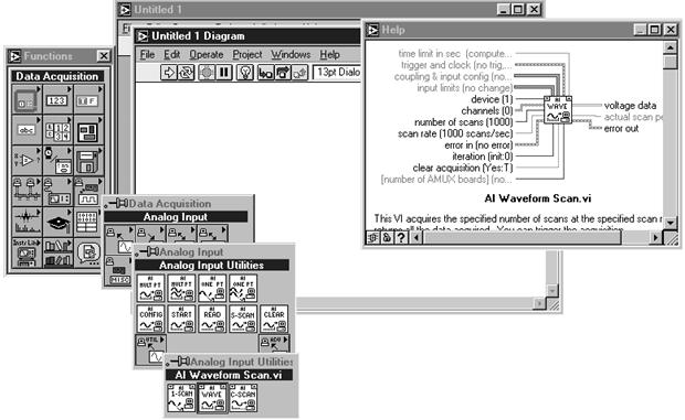
Find out what the difference is so that you will know which one to use. Then put: a data-acquisition module; a power-spectrum module; an index array module; and a numerical constant on the diagram. You'll find the data-acquisition module, which is called AI Waveform Scan.vi, located as in Figure 12. Here's where to find these modules:
- Controls-->Graph Indicators-->Waveform Chart/Waveform Graph (you will need 2)
- Functions-->All Functions-->Array-->Index Array
- Functions-->All Functions-->Numeric-->Numeric Constant
- Functions-->All Functions-->Analyze-->Signal Processing-->Frequency Domain-->Power Spectrum
- Functions-->All Functions-->NI Measurments-->Data Acquisition-->Analog Input-->Analog Input Utilities-->AI Waveform Scan
Notice that the index array module you found has one input which is black and does not match the one in Figure 13. To modify it, first right click on the "AI Wave" and go to select type change it to "Scaled Array". Then get the wire tool and wire up the Array input to the output of the AI Wave. The first input will change from black to outline after you add a constant to the second input of the Array. These changes are necessary because the "AI Wave" module spits out a 2-dimensional array of numbers including a column of voltage values and a column of indices, while we only want a 1-dimensional array of voltage values. Wire up the modules as shown in Figure 13. What module is missing? where should it be wired to? One of the [DBL]'s will turn into a [SGL] after you make some connections. Make sure you know which inputs and outputs to connect on the modules.
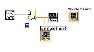
The module labeled "AI WAVE" samples the voltage signal connected to the computer at a fixed rate (default 1kHz), and returns an array of numbers that represent the voltage levels at successive intervals. That is, if the sample rate is $f_s$, then the sample period $\tau=1/f_s$, and the AI WAVE VI returns an array that is $\{V(0),V(\tau),V(2\tau),\ldots,V((n-1)\tau)\}$, where n is the number of points.
Once you have wired up the VI, you're ready to use it to sample signals. Using a function generator (Stanford Research Systems Model DS345), adjust its output to produce an approximately 200 Hz sine wave, 5 Volts in amplitude (10V peak-to-peak). Use a scope to check the output. Then connect the function generator to the Computer Interface(Fig. 22) box, into the connection labeled Analog-input channel 0. Run your VI by pressing the "run" button.
Your two graphs should display the time-series of the signal (it should look like a sine-wave) and the discrete Fourier transform (DFT). We stress that it's the discrete transform because, while it is closely related to the continuous Fourier transform, there are some important differences that we hope you'll discover. The units of the time-series graph are Volts vs. Sample number. What are the units of the DFT window?
The Fourier transform of a sine wave is a delta-function (loosely speaking, a peak). To better see the harmonic content, set the Y axis of the DFT graph to a logarithmic scale, accomplished by right-clicking on the graph in edit mode and selecting y-axis formatting. Why do you see two peaks in the DFT and not one? Now change the frequency. Vary it between 100 and 10,000 Hz. See if you can explain what's happening.
Figure 14: The graph-axes tool-palette
As you experiment with the parameters of the exercise, you may want to change the range of the graphed data. For this purpose, each graph window has its own palette of display controls (Figure 14). These control auto-ranging of the axes, format and precision of the axes, zooming, scrolling and the use of graph markers. See Ch 15 of the LabVIEW User Manual for more information. You may also highlight (with the mouse) and type directly onto the axes scales.
Next, change the waveform from a sine to a triangle at 100 Hz. . Calculate, or look-up in a reference, the Fourier series of a triangle wave. Does the displayed spectrum match what you expect?1 To help you determine the frequencies of different peaks, you should use graph cursors. You can enable them by right-clicking on the DFT window and selecting "show?cursor display." This displays a palette of controls that permits the marking and measuring of values on the graph. See the LabView manual for details.
The harmonics of the triangle wave that occur above the Nyquist frequency, will be aliased. Adjust the frequency of the function generator between 100 and 800 Hz, and familiarize yourself with the operational details of aliasing.
One-dimensional maps: Introductory chaotic systems.
Multi-dimensional differential equations are hard to study. If they are insoluble, only numerical integration is possible. As simple examples of chaotic systems, one-dimensional maps offer an easy way to explore the defining features of chaos.
To familiarize yourself with 1-d maps, you will write a "cob-web" analyzer VI that shows the progress of iterations of the quadratic map (See Figure 15). Be sure to at least glance at §10.2 Ref. 1, to get an idea of what's going on.
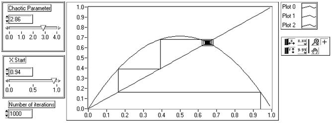
The graph displays three plots. The downward parabola is the quadratic map $f(x)=rx(1-x)$. The straight line is g(x) = x, and the stair-step or "cobweb" is the effect of successively applying the quadratic map to the initial point, x =0.94 . The recipe for producing the cobweb is as follows: Begin with the initial point $x_0$, follow a vertical line up to $f(x_0)$, follow a horizontal line over to the line y =x, you are now at the x-coordinate $f(x_0)$, proceed vertically to the graph of the quadratic map. You are now at the y-coordinate $f(f(x_0))$ Each time you move vertically to f, you have performed a further iteration of the map. Continuing in this way you can explore the long-term behavior of the map as you vary the initial condition and the chaotic parameter.
Making this VI yourself will teach you about arrays, or lists of numbers, in LabView. If you haven't programmed in a computer language before, you should know that each number in an array is indexed starting from 0 to N-1. Here's the part of the cobweb VI that produces the graphs of f and g (Figure 16).
The big square is a for-loop that gets executed 100 times (the constant 100 wired to N). Each time through the loop the variable i increases by 1 (i starts at zero and goes through (N-1)). The quotient $\frac{i}{N}$ is calculated and assembled into an array, which we shall call $x_i$, at the right border of the loop. The function $f(x_i)$ is computed and also accumulated. The array is accumulated by means of the "indexing" feature at the border of the loop. Whenever you connect a wire from the inside to the outside of a loop a border node is formed to control how the data flows. Pop-up on the node to enable "indexing" and the result of each iteration will be assembled into an array. Leave indexing off and only the single number that was calculated last will be passed on.
Outside the loop, the arrays are "bundled" into a form that the XY-graph module will accept: an array of x-values bundled with an array of corresponding y-values. A "bundle" is a LabView data-structure that is a convenient way of collecting several things into one. It basically creates a list of ordered pairs, $\{x_i,y_i\}$ which the program then builds into an array with three such lists. The graph reads these three lists of ordered pairs and plays connect the dots, making three graphs. One graph is made by taking the $x_i$ array and bundling it with itself, producing the graph of y =x. The downward parabola, $y=rx(1-x)$, is made by bundling $x_i$ with $f(x_i)$.
That was the easy part, the graph of the cobweb part is a little harder and requires some discussion beforehand. We've already written a VI, named quad.vi, that calculates successive iterates of the quad map. The VI is located in c:\NLD-chaos\LABVIEW\CHAOS. So let's assume we have a series of map-iterates
$\large m_i= \{m_0,m_1,m_2,\cdots ,m_n\}= \{x_i,f(x_i),f(f(x_i)),\cdots f^n(x_i)\}$
We arrange these values in a way that will let LabView draw the cobweb by connecting the points:
$\large \{x_i,y_i\}=\{(m_0,0),(m_0,m_1),(m_1,m_1),(m_1,m_2),(m_2,m_2),(m_2,m_3),\cdots (m_{n-1},m_{n-1}),(m_{n-1},m_n)\}$
The x-values form a series $\{m_0,m_0,m_1,m_1km_2,m_2,\cdots,m_{n-1},m_{n-1}\}$
which we may form by "interleaving" the $x_i$ array with itself and removing the last two elements. Fortunately, LabView has a function that interleaves arrays and a function that takes an array's subset.
The y-values of the cobweb form a series $\{0,m_1,m_1,m_2,m_2,\ldots ,m_{n-1},m_n\}$
which can also be made by interleaving the $x_i$ array and taking subsets (and replacing one element with a zero). Once you have the two arrays of x's and y's, you must bundle them together and then build an array out of this bundle and the other bundled plots of f and g (see the right side of Figure 16).
Try making the cobweb analyzer yourself. First, understand and make the section in Figure 16. Make the "Build array" icon have only two inputs, and then run the program. It should give you a graph of y =x and y =rx(1-x). Next, expand the "Build array" icon to three inputs and start the cobweb part. Be sure to look at quad.vi to see how it works. You can add a VI into your diagram by going to the functions palette and clicking "Selecting a VI...". You can then treat it as any other module with inputs and outputs. Consequently, all of the inputs in quad.vi will need to show up on your front-panel except for the pre-iterate input which you should just wire with a zero in your diagram. There are lots of different ways to program the cobweb, but you'll probably find the array functions "Build Array," "Interleave 1-D Arrays," "Replace Array Elements," "Array Size," and "Array Subset" helpful. Read what these modules do, and then make a block diagram on paper illustrating how you would use these functions to make the necessary x and y arrays for the cobweb. Then wire it up in LabView, bundle them together as before, and input it into the "Build Array" next to the other two bundles. Be sure to pay attention to whether your inputs/outputs are single elements or arrays of many elements. Some of the module inputs need to be told whether to accept elements or arrays.
Again, try to do this on your own. If you get really stuck, you can look in appendix A of this write-up for hints. Once you have the working VI, you can use it for a variety of things. Observe how the derivative of $f(x_i)$ affects the stability of fixed points (Ref. 1 §10.1). Look for limit cycles, period windows, etc. Change the function $f(x_i)$ to $f(f(x_i))$ or some other 1-d map and observe the same qualitative behavior. To do this, you will have to modify both your program and quad.vi. Save quad.vi as quad2.vi in your directory rather than messing with the original. Try any non-invertible function that takes the unit interval to itself. There are numerous ones in the references: the tent map, the shift map, the sine map, etc. Try to come up with one of your own. Pretty much any function with a range of the unit interval that starts at (0,0) and goes to (1,0) will work. The maps must be non-invertible because there must be some dissipation in the equations [Ott p8]. Try at least one other map and analyze it.
Numerical calculation of Liapunov Exponents
Sensitive dependence on initial conditions is one of the defining features of chaotic behavior. Consider two close initial-conditions, $\xi$ and $\xi +\delta$ evolving in time. If their distance of separation increases exponentially, i.e. $\large |f(t,\xi)-f(t,\xi +\delta)|=\delta e^{\lambda t}$, we say the function f exhibits sensitive dependence on initial conditions. The coefficient is necessarily positive and it is called the Liapunov exponent (see ref. 1, section 9.3 especially the qualifications after fig 9.3.5). As such, if you can calculate or measure , you have a test to determine whether or not a particular system is chaotic. If is not positive, the system is not chaotic.
As previously mentioned, the Liapunov exponents of multi-dimensional systems are the average eigenvalues of the Jacobian matrix of the system (see also Theiler eq's 4-7). So rather than solving an eigenvalue problem on a multi-dimensional system, it's easier to start with a one-dimensional map. The Liapunov exponent for a 1-d map is given by (Ref. 1, p367). Following example 10.5.3 in Ref. 1, write a VI to calculate the Liapunov exponent of the quadratic map as a function of its chaotic parameter . You will probably find it useful to know that the inputs to LabView's arithmetic operators are polymorphic. For example you can wire an array and a constant to the "add" function and the result is a new array whose elements are the old array with the constant added to each of them. Most of the math functions work this way for instance the log function can take an array of numbers and produce an array of logarithms of the numbers (see Figure 17). You will make use of quad.vi again.
The front panel of your finished VI should look something like Figure 18. After you look at the algorithm in Ref. 1, make another block diagram of what you'll want to do and then try it in LabView. You'll probably find a FOR loop helpful. If you find yourself spending more than an hour or so on it, you should look at the solution in the appendix. When you have your working VI, explore the area around r=3.57 especially. What happens when λ--->0 Use your observations to approximate Feigenbaum's ratio δ. Ref.1 suggests 10,000 iterations, but this is a bit excessive, not to mention time consuming. Make sure to have lots of different values for r, the chaotic parameter. Experiment to see what gives you good graphs.
NLSIM.VI: the simulation VI
Before proceeding to real-time NLD systems, you will take some time to run the simulation VI, NLSIM.VI. Open NLSIM.VI. This VI (Figure19) allows you to display the time-series, return-map and power spectrum of a variety of signals. As in all the VI's, press control-H and move the mouse pointer over the elements of the screen to get specific information on how to use the program.

Start the VI, select the cosine function, and focus your attention to the return map. Many dynamical systems are described by a cosine function, for example the simple harmonic oscillator of a mass on a spring: $x(t)=A\cos {(\sqrt{\frac{\kappa}{m}}t)}$. What are the axes of the phase space of this system? What is the shape of the paths in phase space for this system? Is it similar to what you see in the return map? What effect does changing the sample rate have on the shape of the trajectory? When you increase the sample rate, why does the return map narrow around the line y=x? What happens if the sample rate is a multiple of the frequency of the cosine? Now try the function $\cos {(\omega_1t)}+\cos {(\omega_2t)}+a\cos {(\omega_1t)}\cos {(\omega_2t)}$. The return map for this function is more complicated: When a is zero, it's a two-dimensional uncoupled harmonic oscillator and its trajectories are confined to a torus in phase space (c.f. Ref. 1, §8.6). What conditions are necessary for the return-map to show a projection of a torus and not a cycloid? Be sure to explain what you're seeing in the Time Domain and Frequency Domain. Is it chaotic?
Now select the Quadratic Map function and set the parameter r=2.8 . The return map should show a single point. Increase r to about 3, the map will bifurcate, and you should see two points on the return map. Continuing to increase r will produce successive bifurcations and finally chaos at r=3.5. One dimensional maps like this one are good analogs to Poincaré sections and when you sample the real NLD systems synchronous to their driving forces, you will see the same behavior. So it pays to spend some time here to really figure out what's going on. Be sure to compare this map with your cobweb VI at the same value of r. Also look at the quadratic map's bifurcation program.
Take a look at the Henon Map. Play with the non-linear parameter between 0 and about 1.4. What is that funky thing in the Return Map? Look at the Henon map's bifurcation program as well.
Continuous-time systems- PN Junction
Now we're ready to proceed to real-time continuous systems. At present there are two driven NLD systems at the experiment station: The bouncing ball circuit and the PN-junction. For both these driven systems, the basic set-up is the same: The computer controls the driving amplitude and measures the system's response. Both circuits, as well as most of the supporting electronics are located behind the large panel marked "Nonlinear Dynamics Laboratory."(see fig. 20)
The drive oscillator is an Stanford Research System Model DS345. It is fed into the external reference pin $\large V_{ref}$ of the DAC on the computer. Recall from your basic electronics experience that when you set a DAC to a specific level, e.g. j out of a maximum of N, the DAC outputs a voltage equal to $\large V_{DAC}=V_{ref}\frac {j}{N}$. Thus, if $\large V_{ref}$ is a sine-wave varying in time, the DAC outputs a sine wave of attenuated amplitude. The computer modified sine-wave is then fed to the NLD system under study. The NLD system's response is sent to the ADC input of the computer where it can be sampled either synchronously or asynchronously with respect to the driving frequency. When sampling is performed asynchronously, an internal timebase (not shown) is used. Synchronous sampling is achieved by a "strober," which sends TTL pulses to the EXTERNAL TRIGGER pin of the ADC whenever the drive signal achieves a certain phase (adjustable as "Pulse delay" on the NLD box) in its cycle. The sine-wave is also connected (via the square-wave converter on the NLD box) to the computer's timer pin (labeled GATE0) for computer measurement of the drive frequency.
Turn on the system with the switch located at the top of the rack.
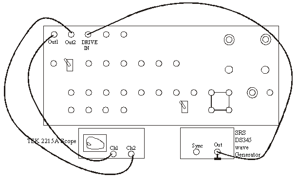
Let's begin with the PN Junction: Make the following connections referring, in addition to Figure 21:
- $\bar {TTL}$ to the back of the Tektronix 2215A scope
- Set the SRS DS345 to f= 3500 Hz and 10 volts peak-to-peak output.
- Set the STROBE PHASE CONTROLLER "DELAY RANGE" to 30 ;μs and "ADJ" to 0.0 (fully CCW)2
- Set the STROBE PHASE CONTROLLER "WIDTH RANGE" to 3 μs and "ADJ" to 0.0 (fully CCW)
- Set PN JUNCTION DRIVER "GAIN" to 0.0 (fully CCW).
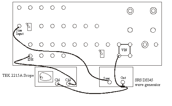
You should now see a horizontal line on the scope. Increase the PN JUNCTION DRIVER GAIN and the scope should display an ellipse. Having connected $V_o(t)$ and $V_s(t)$ (recall the notation of the introduction) to the x, y axes of the oscilloscope(remember to put the time dial on x.y). The displayed graph is a plot of I vs. $V_{os}\cos {(\theta)}$, a two-dimensional projection of the system's path in phase space.
At such a low driving amplitude, the diode is responding linearly: The diode current is periodic at the same frequency as the drive oscillator with a small phase offset. Observe the behavior as you increase the DRIVER GAIN- it should follow the discussion of the pn-junction earlier in this write-up and the video.
The scope highlights sections of the plot according to the STROBE PHASE CONTROLLER adjustments. Make sure the scope intensity is not too bright and you should be able to see the dots corresponding to points of constant phase of the drive. Recall that the state-space for this system is $(I, V_d,\theta)$ so a set of points sampled at a constant θ constitute a Poincaré section, a subset of state space that slices the attractor non-tangential to the trajectories. The Poincaré section will contain as many dots as there are loops. Changing the DELAY potentiometer moves the slice along the attractor. When you sample asynchronously, the computer will sample coincident with the dots.
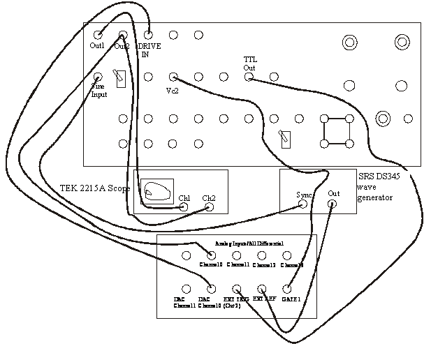
Now let's include the computer. All of the connections to the computer are made through a single box, called the Computer Interface Box (fig. 22).
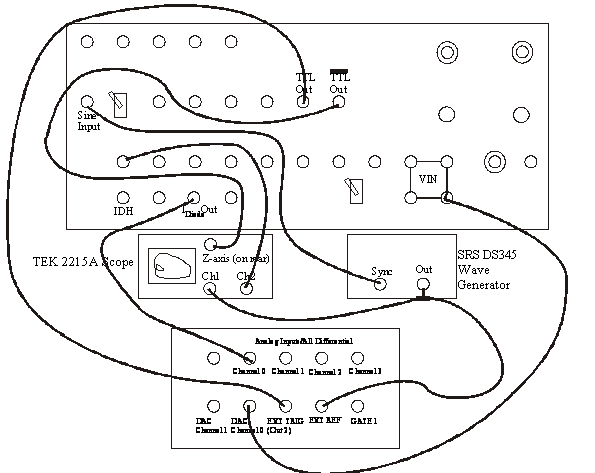
Disconnect the SRS DS345 from Vin and make the following connections, in addition to looking at figure 23.
- SRS DS345 50Ω "FUNCTION" output --------------------------to COMPUTER "EXT REF"
- COMPUTER "DAC0"------------------------------------------to PN JUNCTION "Vin"
- PN JUNCTION "Differential Idiode out"-------------to COMPUTER "AINP DIFF Analoginputs/all differential) Channel 0"
- STROBE PULSE GENERATOR "VC2"------------------------to COMPUTER "GATE 1"
- STROBE PULSE GENERATOR "TTL OUT"----------------------to COMPUTER "EXT TRIG"
- "SINE INPUT" switch set to --------------------------------Off
- set the switch below AUX in/out to "INT"
Start LabView and load NLDGEN. You should see a display similar to Figure 24.
This VI controls the drive amplitude, collects a sample of data points, and presents three different views of the response: a time-series, Fourier power spectrum, and return-map. We suggest you use ~30kHz for the sampling rate. The more points you take in your sample, the better your DFT resolution will be, but the longer the computer will take to calculate and display. So to start, select 256 points. You should make sure that the product of "Number of points per value of V" and "#" of points" does not exceed 231 - 1. Vary the drive amplitude and estimate Feigenbaum's ratio based on the system's bifurcation points. Compare the return map to the picture you see on the scope. There are two other features of this VI: You can save the data to a file, and send the data to a subroutine that calculates information dimension. We'll discuss these options later.
Before moving on, open up pnbifur.vi, which will allow you to view the bifurcation diagram for the PN-junction. Leave the computer and hardware in the same configuration as for nldgen.vi, except turn the knob for PN-JUNCTION DRIVER GAIN all the way up (CW). You should also look at the real-time output on the scope, so also hook the output on the SRSDS345 to the X-channel on the scope, and the IDH output on the PN-JUNCTION DRIVER into the Y-channel, just as before. Run pnbifur.vi and look at several different ranges of V. You should make sure that the product of "Number of points per value of V" and "#" of points" does not exceed $2^{15}-1=32767$.
Bouncing Ball
Let's now turn our attention to the bouncing ball circuit (BB).
- Connect the SRS DS345 "FUNCTION" output to the "DRIVE IN" on the panel.
- Connect BOUNCING BALL "OUT 1" to the Tek 2225 scope CH 1.
- Connect BOUNCING BALL "OUT 2" to the Tek 2225 scope CH 2.
Set the DS345 to ~50Hz and ~15V peak-to-peak (just turn the knob to about half-way in its range). Look at each channel in time. They should both be sinusoids. Put the scope in X-Y mode and you will see the system's phase portrait. The circuit is fully described in the reprints so we will only summarize it here: The circuit simulates the dynamics of a ball bouncing on a vertically sinusoidally driven table. One output is ball velocity, one is ball position (height from a fixed reference). When the table frequency and amplitude are small, the ball basically stays on the table and the phase portrait is that of an harmonic oscillator. Increase the drive frequency and you should see the phase-portrait begin to change. The phase-portrait becomes jittery and then it should jump to behavior that is periodic at twice the drive frequency. Take some time to understand the simple behaviors of the phase portrait: Which axis is velocity? Which is position? Why is the initial plot an ellipse? What's happening just as you increase the drive frequency but before the plot becomes jittery? Try varying the drive voltage.
Now we're ready to hook up the computer. Make/check the following connections, referring to fig. 26:
- Disconnect the PN-JUNCTION Vin from COMPUTER DAC0
Connect . . .
- DS345 "FUNCTION" output-------------- to COMPUTER "EXT REF"
- DS345 "SYNC" output--------------- to STROBE PULSE GENERATOR "SINE INPUT"
- COMPUTER DAC0--------------- to BOUNCING BALL "DRIVE IN"
- BOUNCING BALL "OUT 1"-------------- to scope CH1
- BOUNCING BALL "OUT 2"----------------- to scope CH2 and COMPUTER "AINP DIFF CH0"
- STROBE PULSE GENERATOR "VC2"--------- to COMPUTER "GATE 1"
- STROBE PULSE GENERATOR "TTL OUT"--------- to COMPUTER "EXT TRIG"
- Set the DS345 to f =90Hz and full amplitude output.
- Run the NLDGEN VI and start by sampling 256 points at 500 Hz
What is fundamentally different about the chaotic behavior of the bouncing ball circuit when compared to the PN-Junction? (Hint: What would the bifurcation diagram for this circuit look like? Does it even have one?)
Information dimension
Figure 27: Data from the Quadratic map, analyzed by the information-dimension VI.
Chaotic systems have fractal attractors and a commonly measured quantity is the attractor's information (or correlation) dimension (Ref. 1, §11.5, Ref. 4, pp1062-1063, pp1066-1070). The correlation dimension measures how the state-space "mass" of the attractor scales with length. CALCCORR.VI computes C(N,ε) , the number of points within a distance ε of each other, for increasing embedding dimensions and then displays $\log_{2}C(N,\epsilon)$ vs. $2\log_{2}\epsilon $ (Figure 27). The slope of the linear region of the plot is then 1/2 times the information dimension. See the article by Theiler for full details and Ref. 9 for a simple application of these concepts.
As an introductory exercise, do the following: Run NLSIM.VI and CALCCORR.VI. Select "Random number generator." Choose 2048 points and press the "Send data to the info-dimension VI" button. Press "Calculate" in CALCORR. When the calculation is done, use the graph cursors to estimate the slope of each line. How does each slope compare to the line's embedding-dimension?
The data calculated by CALCCORR.VI can be saved to a data file for more accurate linear fitting. Simply press the "send data to a file" button, name the file, and open it from within Excel (or copy it to a disk and take it to your favorite software). You should measure the information dimension of the PN-junction and the Bouncing Ball circuit for varying driving amplitudes and frequencies. Are the values what you expect?
What your report should contain
Your report should be an introduction to NLD and Chaos and a presentation of experimental results. Most of this material about chaos is unfamiliar to the majority of undergraduates. Thus your goal should be to illustrate the concepts set forth in the reading by relating them to what you did in lab.
The results you should present are at least the following: Experimental confirmation of the bifurcation route to chaos. The value of Feigenbaum's scaling constant α and δ measured from a variety of sources. What does Feigenbaum mean? The information dimension of the attractors of the PN-junction and the Bouncing Ball circuit as compared to that of conservative (Hamiltonian) systems. How do the Fourier Transform, the frequency spectrum, and the power spectrum differ?.
Be sure to answer the questions posed in the write-up and include your answers to the pre-lab.