Pages in this Lab:

• CW NMR (Lab Manual)
• Pulse NMR (Current Page)

 

• Contents 1 Introduction 2 Prerequiste Reading Materials 3 Experimental Procedure 4 The Report 5 Pulsed NMR Equipment 5.1 Sample Coil 5.2 RF Pulse Section 5.3 Detection Block 6 Pulsed NMR Setup 6.1 PRE-Amp SRS SR560 6.2 10LA Amplifier: 6.3 Tektronix 2230 Digital Oscilloscope 6.4 DG535 Four Channel Digital Delay/Pulse Generator: 7 Pulsed NMR Appendices 7.1 Pulsed NMR Appendix I 7.2 Pulsed NMR Appendix II 7.3 Pulsed NMR Appendix III 8 NMR Scope Program

Introduction

The study of nuclear magnetic resonance or nuclear induction has explained many characteristics of atomic systems. The usual approach is to observe the nuclear resonance of an ensemble of nuclear moments in a large static magnetic field as a function of a slow change in this field. Meanwhile, a small radio frequency field is applied continuously to the nuclear sample in a direction perpendicular to the large field. This is the method of continuous wave nuclear magnetic resonance, or CW NMR, an experiment which you have already completed. An alternative method to this steady state or slow passage technique is one in which the radio frequency field is applied to the sample in short intense pulses, and nuclear signals are observed after the pulses are removed. The effects which result are comparable to the free vibration or ringing of a resonant cavity. It is this latter technique which is used in this pulsed NMR experiment. The purpose is to gain further experience with nuclear resonance and to measure relaxation times T₁ and T₂ for protons in several solutions.

Prerequisite Reading Materials

Watch the Pulsed NMR Video.

 

1. E. L. Hahn, "Free Nuclear Induction", Physics Today, November 1953. \#QC1.P447
2. R. G. Brewer and E. L. Hahn,"Atomic Memory", Scientific American 251.50 (1984). \#T1.S5
3. E. Fukushima and S. B. Roeder, "Experimental Pulsed NMR, a Nuts and Bolts Approach", Westview Press (1993).
4. E. Hahn, Spin Echo
5. Pulsed NMR; Physics 322, Physical Measurements Laboratory

Experimental Procedure

1. Use the set up for CW NMR to determine the orientation of the sample in the magnetic field that maximizes the resonance. Record the resonance frequency TO ALL THE FIGURES GIVEN ON THE FREQUENCY COUNTER. It is very important to record the resonance as accurate as you can for a sample, as the signal generator in the pulse NMR experiment will need to be tuned to send in a resonant frequency and is very sensitive. Replace the sample holder with the one for the pulsed NMR, making sure that the sample will still be at the same location as before. You can fine tune this later, but get as close as you can to the location of the CW NMR head.
2. Check out the equipment by identifying each component shown in Fig. 1. Turn everything on, set the oscillator frequency to the proximity of the resonance frequency, for example 16.07x,xxx MHz (you may have to set it correctly to within 100 Hz), the approximate Larmor frequency (Hint: same as for CW), and the pulse frequency to 1 Hz. Refer to the end of this write-up for a complete list of settings for all of the equipment in this experiment.
3. This experiment uses the "Pulsed NMR Rising Edge" function in the Labview program "NMR Scope2.0.vi." Simply switch the setting in Labview to this to perform this part of the experiment. You will also want to be in "TY Average" mode, which plots time on the x-axis and the Y input on the y-axis. In the averaging mode, the top trace plots the data in real-time, and the bottom averages the signal over time. You will need to look at the bottom (averaged) trace to see the pulsed NMR signal clearly, the top trace will only give you a reference for changing settings but contains a lot of noise and is hard to see the signal.
4. Put a glycerin sample into the holder inside the magnet, and see if the correct signal (example given later in the write-up) appears. If not, it will be helpful to "follow" the signal through the components, using the block diagram as a guide. To follow the signal, simply connect a BNC cable to Ch. 1 of the scope and look at the pulse at various points in the setup. At some points it is easier to view the pulses using the "A Source INT" trigger setting, which uses internal triggering, and other times it will be easier to see the pulse by plugging in the T0 output from the pulse generator into the "EXT INPUT" on the scope, and flipping the A SOURCE switch to "EXT." From here, adjust the frequency, Ch. 1 amplitude, etc. until the pulses are visible. Make sure the pulses are visible throughout the block diagram where they should be. Optimize the signal by moving the PNMR head in the magnet.
5. Vary the oscillator frequency and observe the signal and how it changes. Also vary pulse widths, delays, offsets, etc. to see their effect on the signal, and become equipped with making the signal how you want it.
6. Once an optimal signal is obtained, T₁ and T₂ can be measured. These values can be obtained in a few different ways, one of which is mentioned in the video: take the Fourier transform of the signal, and T₁ and T₂ have a simple relationship to the FWHM of the peak in the frequency domain.

Another way to measure T₁ and T₂ is from the Labview data directly. For T₁, once a good spin-echo signal is obtained, vary the pulse separation (time between pulses) and record the amplitude of the spin-echo signal. Eventually, with large enough separation, the spin-echo signal will diminish and eventually vanish. Take data out to this point, and plot it in MATLAB  (or your favorite data processing language). Once plotted, use the curve fitting tool to fit an exponential function of the form $A*e^{-bx}$ to the curve. The parameter b is just the inverse of T₁.

T₂ is obtained from the plot AT RESONANCE directly. As mentioned at the end of the pulse NMR video, when the oscillator frequency is tuned finely to resonance, the "wiggles" in the ringing from the first pulse and the spin-echo effect will turn into envelopes of the spin-state decay. From above, you should have already obtained a plot (or at least written down the settings) that produce resonance and give these envelopes. Once you have good resonance data, upload it into MATLAB and plot the section of the growth of the spin-echo envelope. It will have a positive slope, which is reversed from what is shown in the video, but that is ok. Try to only use data points from the part of the spin-echo signal that adhere to an exponential curve. After singling out these data points, again use the curve fitting tool in MATLAB to fit an exponential to the data. Like before, T₂ will simply be the inverse of the b factor given.

7. Put a water sample in the magnet, and reproduce its curves on and slightly off resonance. Make sure that the pulse frequency is long enough. Water has a much longer relaxation time than glycerin. Try other samples if they are prepared and ready to use.

The Report

• Use the NMR Program and get data for T1 and T2.

This experiment is largely a show and tell one, because there are no detailed calculations or curves to be plotted, except for the transform and/or the exponential curve fittings. Explain in your own words what is happening, and account for the signals at each point. Explain the appearance of the spin echo signal and why its shape is different from the other pulses. Explain the changes that occur as you vary the oscillator frequency. Explain why digital storage is required to see the signals in some cases. Compare the signals for the different liquids, and explain.

Pulsed NMR Equipment

Sample Coil

This Laboratory uses a simplified version of the "single coil" pulsed NMR spectrometer. The basic elements of this spectrometer are the same as those found in most commercial and home-built research spectrometers. The difference is mainly in the sophistication of the data acquisition hardware, and in the quality of the magnet. A commercial superconducting NMR magnet provides a 10 tesla magnetic field homogeneous to 1 part in 10⁹, while ours provides a 0.3 tesla field homogeneous to about 5 parts in 1000. The design is referred to as a single coil spectrometer because a single radio-frequency coil wrapped around the sample is used for excitation of the precession of the nuclear magnetization by application of a short pulse of RF current to the coil, and also is used to detect the subsequent Larmor precession of the nuclear spins by detecting the voltage that their oscillating flux produces across the coil$\!\,\left ( V = - \frac {d \phi} {dt} \right )$. A single coil produces a stronger signal with less noise as compared to the two-coil method used in the CW NMR experiment. The spectrometer can be separated into two blocks: the electronics that produces the oscillating RF magnetic field pulses at the sample which induce the nuclear precession, and the electronics necessary to detect this precession after the RF pulse. These two sections are called the "RF pulse" block, and the "detection" block.

A schematic diagram of the Pulsed NMR apparatus is shown in Figure 1 below.

Follow the diagram in Figure 1 while reading this general discussion of how the system operates. You can also follow the circuit and apparatus displayed at the experiment location. [Note: It is unfortunately true that the labels on the apparatus parts are not standard in other branches of electronics, so the names, which are in the RF set of electronic terms, sometimes are misleading.]

Start with the CW RF oscillator that operates at the approximate Larmor frequency of 16.07x,xxx. MHz you found in the CW part of this experiment. The output is split into two parts, one of which is used to pulse the NMR head, and the other to serve as a comparison frequency for the output signal from the NMR head. Follow the branch that goes to the RF Gate Mixer M1 which is labeled LO. A 50 microsecond gate from the Pulse Generator goes into the same mixer at port IF. The output labeled RF is 16.1 MHz RF modulated with a 50 microsecond on-off gate, at a modulation frequency of about 1 Hz. These RF pulses go through an amplifier, a Noise Blocker, Impedance Matching Capacitors, and finally into the Pulsed NMR Head and the Sample inside it.

Out of the NMR Head comes the output signal, which is blocked by the Noise Blocker but continues to the quarter-wave Delay Line, past the Protection diodes, through the Low Noise RF AMP into one port of the Mixer M2. Into another port goes the 16.1 MHz RF reference signal split off from the CW RF Generator. The output of the mixer is the small difference frequency between the 16.1 MHz reference and the signal from the NMR Head, which is at the Larmor frequency. The output passes through a Low Pass Filter, an amplifier, and finally into a digital scope.

Now for the details; In the NMR Head, both the RF Pulse and Detection blocks share the tuned RF coil wrapped around the sample. The detection and excitation are most efficient when the coil is tightly wrapped around the sample. The coil is ten turns of thick copper wire wrapped around an insulated form that the sample tube is inserted The inductance of the coil is about 1 microhenry. The coil and a 10 - 100 pF capacitor form a series LC circuit tuned about one MHz below the finally desired Larmor frequency expected for the sample in the applied static field H_o. The tuned LC circuit is in an aluminum box, to provide shielding from stray RF pick-up. The whole box slides snugly into the magnet. No magnetic materials are used in this part of the spectrometer. Be careful of the leads of the capacitor! A short 50-ohm coax cable comes out of the magnet to the variable tuning capacitors.

At resonance, the series LC circuit has a real impedance of less than one ohm. The functions of the two tuning capacitors are to transform this impedance to the 50 ohm impedance expected by the rest of the electronics in the two blocks, and to tune the resonant circuit so that this impedance matching occurs at the desired Larmor precession frequency. If this impedance matching is not done well, there is no hope of detecting an NMR signal from this apparatus. Since it requires some specialized RF test equipment to set the impedance properly, students, GSIs, staff, and faculty must avoid fiddling with this setting. With two knobs on the two variable capacitors that must be set exactly to see an NMR signal, it is a bad idea to touch them even as a last resort when nothing else produces a signal. It is far better to spend your time searching for the proper RF test equipment to check the impedance match than to meddle with the capacitors. Also, changing the length of the coax from the LC circuit to the variable matching capacitors greatly alters the impedance match. Once a given cable is chosen, it should not be changed. See Don if you need help.

For the record, these two 10-300 pF variable capacitors can be set by disconnecting them and the LC circuit from the rest of the apparatus and hooking them up to an RF vector impedance meter set to the Larmor frequency. This procedure should not be done by the student, but only once (and we hope they will be left alone forever after) by a GSI or Professor. The vector impedance meter measures the real and imaginary parts of the impedance of a passive circuit. The real part should be adjusted to 50 ohms, and the imaginary part to 0 ohms or the magnitude to 50 ohms and the phase angle to 0 degrees). Another method of matching the impedance requires a RF sweep generator and a magic Tee directional coupler (see Pulsed NMR Appendix II and III).

RF Pulse Section

This section describes how the RF pulsed magnetic field (H1 ) is applied to the sample. The RF oscillator produces about one volt peak-to-peak CW at the desired Larmor processional frequency. This CW RF is gated into pulses by the mixer M1. When the CW RF goes into the local oscillator port of the mixer, the output at the RF port of the mixer is zero when no voltage is applied to the IF-port (the Intermediate Frequency, which is DC in this case), and is a maximum when a DC voltage applied to the IF- port is sufficient to inject a 40 mA current into the port. The input/output impedance of the mixer ports is 50 ohms. The mixer can therefore be used as an RF gate by driving the x-port with a pulse generator capable of supplying 40 mA at 50 ohms in its high state. [Notes: most TTL pulse generators cannot do this. The two mixers used in this apparatus are double balanced mixers of modest quality.\] The output of the mixer RF-Port is a 1 volt peak-to-peak burst of RF about 50 µseconds long. A typical repetition rate is 0.5 Hz; it must be less than 1/T₁ for the sample. The pulse should be nice looking and square. It is important that there not be significant CW leaking through the mixer when the pulse is off. The RF pulse is then amplified by the RF power amplifier, whose output is an RF pulse about 40 volts peak-to-peak into 50 ohms, about 5 watts of power during the pulse. Examine the pulse to make sure there is no CW RF present between the pulses. Power amplifiers are noisy and one of the purposes of the crossed diodes following the power amplifier is to block this noise and keep it from entering the detection block.

After the RF power amplifier and the crossed diodes, the pulses go into the tuned circuit at point "C" of the diagram. Because the matching capacitors provide an impedance transformation from the tuned LC circuit to 50 ohms, and the output impedance of the power amplifier is 50 ohms, there is no reflected RF power and all of it is dissipated in the residual resistance of the copper coil. For reasons that will be discussed shortly, no RF power travels down into the detection block at point "C" even though it is also connected to the power amplifier. If the Q of the LC circuit is 50 (typical), the inductance L is 1 micro henry, and the LC circuit is tuned to 13 MHz, then the losses in the circuit give an effective resistance R determined by

$\!\, Q = \frac { \omega L} {R}$ or $\!\, R = 1.6 ohms$

So the capacitors transform an impedance of 1.6 ohms (real, on resonance) into 50 ohms, a ratio of 31, (50/1.6). The current in the coil is therefore 31 times larger than the 0.8 amperes seen into 50 ohms, and the voltage across the LC circuit is 1/31 the input voltage (power conserved). The RF current in the coils is therefore about 25 amperes rms, which produces a field H₁ of about 1 gauss rms in the 1 microhenry coil 6 mm in diameter (H₁ = LI /A, where A is the cross sectional area of the coil).

Significant RF power from the amplifier is prevented from going into the detection block of the circuit by the quarter-wavelength cable $\left ( \frac {\lambda}{4}\ \right )$ and the crossed protection diodes. Just as for organ pipes or any resonant tube, an open-ended quarter-wave coaxial cable driven with a frequency $\frac {c} {\lambda}$ has a low voltage, high current node (short circuit) at the driven end. It is therefore possible to short circuit and destroy a RF oscillator or power amplifier simply by accidentally hooking an unconnected (unterminated) quarter-wave cable to it! Proper terminations are important always, before turning on any power! Conversely, a quarter wave cable shorted at one end presents an open circuit (high voltage, low current) node to the driving end. A quarter-wave cable transforms a short circuit to an open circuit, and vice-versa. So, when the power from an RF pulse travels down the quarter-wave cable in this apparatus and starts to turn on the protection diodes at the far end of it, the diodes appear as a short circuit at one end and an open circuit at point A. RF power flows into the 50 ohm impedance presented by the LC circuit rather than the high impedance open circuit presented by the cable and diodes.

Detection Block

Following the RF pulse, the nuclear magnetization is tipped into a coherent superposition state. The nuclear magnetization vector is tipped away from its equilibrium value (along H_o z). The pulse is now off the axis, and the spins are free to precess about H_o at the Larmor frequency $\!\,\nu_o$. This "free precession" induces a voltage across the coil. If the RF pulse tips the spin magnetization by 90 degrees into the xy plane (such a pulse is call a "90 degree pulse" or " $\!\, \frac {\pi}{2}$ pulse", then the magnetization vector M precesses in the xy plane;

$\overrightarrow {M} (t) = M_o \left ( \sin \left ( \omega_o t \right) \hat {x} - \cos \left ( \omega_o t \right ) \hat {y} \right ) $

If the axis of the coil is along the $\hat {x}$ direction, then the freely precessing spins induce a RF voltage across the coil. Eventually the spins dephase (lose coherence) with a time constant T₂^* (about 100 µsec) and the induced voltage decays. The NMR signal after a single pulse is referred to as a "Free Induction Decay", or FID. The goal of the detection block of the apparatus is to detect this small RF voltage which occurs within the 100 microsec time following the large RF excitation pulse. The RF power generated by the spins during the FID flows exclusively into the detection block and not into the output of the power amplifier, since the FID voltage is much less than the 0.6 V needed to turn on either set of crossed diodes. The low-noise amplifier amplifies the FID. It has a gain of at least 60 dB and a 50 ohm input impedance. Note that the impedance matching capacitors insure that the impedance at point "A" is 50 ohms with the quarter-wave coax disconnected, so that all the RF power generated by the spins during the FID is effectively coupled into the detection amplifier.

The NMR signal Free Induction Decay after the low noise detection amplifier is an oscillating RF voltage at the Larmor frequency (about 16.5 MHz) that decays in a time T₂^* of about 100 microseconds. If the output of the detection amplifier were plugged into an oscilloscope, the signal would be lost in the noise. A factor of about 100 in signal-to-noise (S/N) can be gained by using the heterodyne detection scheme employed after the detection amplifier. This is true because just plugging into a 100 MHz oscilloscope lets in a 100 MHz bandwidth of noise while we are only interested in about a 10 kHz bandwidth around the Larmor frequency $\left ( \nu_o \right )$. Wisely limiting the bandwidth of the detection is necessary to see a pulsed NMR signal. The bandwidth reduction is done here by the heterodyne detection technique. A mixer and local oscillator close to the Larmor frequency of the spins, in this case the same oscillator used to generate the RF pulses, is used to mix the FID signal down to near DC frequencies of 100 kHz or less. The low pass filter with a cut-off of 50 kHz then rolls off all undesired frequencies, slope of 6 dB/Octave at the 3dB point. The low-pass filter sets the bandwidth of the measurement. Remember that the spins always precess at the Larmor frequency, while the RF oscillator used to form the pulses just needs to be set to a frequency near resonance with the spins. The mixed-down (after the mixer M2) FID oscillates at a frequency $ \left ( \nu_o - \nu \right ) $. This difference frequency is typically between 1 and 50 kHz, which is within a few NMR line widths. Figure 3A & 3B below illustrates what the FID looks like before and after the mixer.

Figure 3A: Signal of Free Induction Decay (FID) Before the Mixer

Figure 3B: Signal of Free Induction Decay (FID) after the mixer

After the low-pass filter, the signal can be further amplified with an audio amplifier, and viewed with an oscilloscope. For convenient viewing, the RF pulses should be set to come once or twice a second, but no faster than the nuclear T₁ time scale. Since the pulsed NMR experiment is repeated over and over again, we might as well average the FID signals on a digital scope or a computer. If a computer is used, the FID waveform in the time domain can be Fourier transformed to give the NMR spectrum.To use the computer, make sure the computer-interface box is set up properly: (1) select 'pulse', (2) connect the output from the EG&G PARC 113 pre-amp to 'Y in' and with 50-ohm termination, (3) disconnect any 50-ohm termination at the port 'Trig/Pulse 50-ohm/CW' and place it at the port 'X/Trig CW', and (4) connect the output of the SRS pulse generator to 'Trig/Pulse 50-ohm/CW'.

 

Pulsed NMR Setup

Check that the Equipment is set to the following settings:

PRE-Amp SRS SR560

• Input - A, DC
• LF Roll Off - 0.3Hz
• Gain - 2K (or less watch out for the overload light)
• RF Roll Off - 10KHz

10LA Amplifier:

• This is the RF power amplifier
• Power - FWD
• Knob turned to very top (12 o clock) position.

Tektronix 2230 Digital Oscilloscope

• Input - use either Channel A or B
• A Trigger - (i) use EXT : input from TO of the 535 Delay/Pulse Generator; (ii) use NORM; (iii) for A&B INT, use Channel 1; (iv) for A source : use EXT; (v) A EXT Coupling : use AC. To see the waveform easier, select the STORE mode using the button STORE/NON STORE next to the buttons of ACQUISITION at the top of the oscilloscope.
• Nice settings to start with: 5V/div, 1ms/div

• NOTE: While the digital oscilloscope might be helpful with getting quick signals and might be more familiar than Labview, you want to use the Scope 2.0 program in Labview to acquire data. The resonance signals will be most easily viewed on the built-in averaging feature, and data transfer to MATLAB is simple.

DG535 Four Channel Digital Delay/Pulse Generator:

• Read "Using the SRS Model DG 535 Delay/Pulse Generator in the Pulsed NMR experiment" before proceeding.

Using the SRS Model DG 535 Delay/Pulse Generator in the Pulsed NMR experiment:

We use the DG 535 (henceforth the "pulse generator") to generate voltage pulses of arbitrary duration and timing to switch on and off the 16.5 MHz signal going to the RF power amplifier. The duration and timing of these bursts of radiofrequency radiation determines the behavior of the nuclear spins.

Find the Menu section on the front panel of the pulse generator. Press the Trigger button. You will see a menu that looks something like this:

Int Ext Ss Bur Line

The underscore under the I in Int is the cursor, which you can move with the left and right arrows on the front keypad. If the cursor is not under Int, move it so that it is. When on the Int setting, the pulse generator will send a step to the trigger output (T0) at a rate determined by an Internal clock. Press Trigger again. You will see a menu that looks something like this:

Rate = 6.000

This is the rate at which trigger pulses are sent on the T output in pulses per second. Now the cursor indicates which of the displayed digits you are editing. Use the right and left arrows to move the cursor, and the up and down arrows to change the digit values.

Press the Delay button. You will see a menu that looks something like this:

A = T + 0.008 000 000 000

This means that 8 ms after each trigger pulse, the pulse generator will send a step to the A output. Press Delay again. You will see a menu that looks something like this:

B = A + 0.000 055 000 000

This means that 55 microseconds after the step is sent to A, a step will be sent to B. The 'A +' means that the B output is delayed relative to A. You could change this so that B is delayed relative to T (or C or D) by editing the A just like you would edit the numbers.

Continuing to press Delay allows you to set the delays for channels C and D. Note that C should be timed relative to A, and that D should be timed relative to C.

In addition to the step outputs A,B,C and D, there are four pulse outputs. The output labeled AB puts out a high voltage only for the period between when a step is sent to A and when a step is sent to B. I.e., with the settings above, it turns on at time T+8ms and turns off 55 microseconds later. Channel AB is the inverse of AB. The CD pulse outputs are programmed just like the AB outputs.

• Good values to start with for the delay function are:

A = T+ 0.008000

B = A+ 0.000055

C = A+ 0.003965

D = C+ 0.000110

Here CD pulse (D = C+ 0.000110) is twice as long as AB (B = A+ 0.000055) pulse, separation between two pulses is much bigger than both of the pulse widths (C = A+ 0.003965), and 3ms after a trigger pulse (A = T+ 0.003000) the generator sends a step to the A output. (If a 55 microsec wide AB pulse does not work, then try to increase it and the CD pulse by a factor of two. Also, if you are not getting a good signal, try making the width of the CD pulse the same as AB, e.g. 0.000055s).

The Output menu allows you to specify the high and low voltage levels for each of the steps and pulses, as well as the expected load on the outputs. Here are some good settings to start out with:

T: High-Z / TTL / Normal

AB 50 W / Var / Amplitude = 1.40V / Offset = -0.5 V

CD 50 W / Var / Amplitude = 1.40V / Offset = -0.6 V

A,B,C, and D aren't used, so their output settings don't matter.

The trigger output should go to the trigger input of the scope and the AB and CD output should be connected like this:

The output stages are such that if the output are connected, the voltage produced is the sum of the voltages programmed in for each channel: i.e. a baseline of -0.5 V with two pulses rising to +0.5 V. Thus the pulse sequence looks like the following. (Note that this drawing is not to scale. Typically the pulse separation is much longer than the length of either pulse.)

Once you have everything set up and you have a decent signal, try these:

A. Excitation level as a function of "pulse area."

An on-resonance radio-frequency pulse will "tip" the average magnetization vector away from the applied DC magnetic field by an angle which is known as the "area" of the pulse. The area of the pulse is proportional to the integral over time of the RF field strength, and a pulse which tips the magnetization to exactly opposite its original value has an area of $\!\,\pi$ (it's called a $\!\,\pi$-pulse). If the average magnetization starts in the z-direction, then after a pulse of area $\!\,\pi$, the component of the magnetization in the x-y plane will be proportional to $\sin \left ( \theta \right )$. To see this experimentally, tune the oscillator as close to resonance as you can. On exact resonance there should be no wiggles in the free-induction decay. Next, vary the duration of the first pulse and record the height of the peak of the free-induction decay signal as a function of pulse duration. Note the duration of the pulses which correspond to maxima and minima $\!\,\left ( \frac {\pi}{2}, \pi, \frac {3\pi}{2} \right ) $

B. Pulse-Induced Transparency.

Immediately after a $\!\,\frac {\pi}{2}$ pulse, the magnetization has been tipped into the x-y plane, and it induces a voltage in the pickup coil as the nuclei precess. As the nuclei get out of phase with each other due to inhomogeneities in the magnetic field, we can think of each nucleus as being still tipped in the x-y plane and precessing, but pointing in random directions so that on average they induce no signal. The average magnetization is zero. If we now apply any pulse at all, we will not see a free induction decay (FID), because for every nucleus pointing in some direction, there is another nucleus pointing in the opposite direction, canceling its field. This collection of nuclei is transparent. Check this experimentally by applying a $\!\,\frac {\pi}{2} $-pulse and then several milliseconds later another pulse. Does the FID signal after the second pulse depend more on the duration of the first or the second pulse? Why does the FID not completely disappear?

C. Spin Echoes.

Construct a pulse sequence which consists of first a $\!\,\frac {\pi}{2}$-pulse, then several milliseconds later a $\!\,\pi$-pulse. The nuclei that dephased after the first pulse should re-phase and produce an echo of the initial FID. Change the spacing between the two pulses and note the behavior of the echo. There are two characteristic times in this situation. T₂, the rate at which the average magnetization decays away due to dephasing can be measured from the FID, and T₁, the rate at which the magnetization of a single nucleus is lost can be measured from the decay of the echo as a function of pulse spacing.

Pulsed NMR Appendices

Pulsed NMR Appendix I

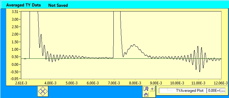
Glycerin sample slightly off resonance. Oscillator frequency set to 16.04999MHz, and the rest of the settings set to the values given above. Do not be concerned with the bump after the second pulse.

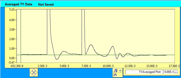
Glycerin sample on resonance. Notice how the wiggles from before are gone and instead there exists two envelopes that give the decay times. Do not be concerned with the bump right after the second pulse. Oscillator frequency set to 16.057970MHz, with the rest of the settings set as specified above.

Pulsed NMR Appendix II

Pulsed NMR Appendix III

 

NMR Scope Program

How to transfer data from the scope to the computer.

Setup:

First we need to make a connection between the computer and the oscilloscope. To do that, locate the aluminum box labeled Computer Interface Unit. Connect a 50-ohm terminator to the X input (X/Trig CW). Connect the Y input (Y In) with the output of PRE-AMP with 50-ohm termination. Connect the output of the SRS pulse generator to the Trig/Pulse 50-Ohm/CW with 50-ohm termination. Don't forget to turn on the Computer Interface Unit.

Now we are ready to use the computer to transfer the data.

NMR Scope Program

The program we are going to use to transfer the data is called NMR Scope. To get familiar with the program you might want to follow the following simple exercise.

On the desktop you will find an icon NMR Scope. Double click on that icon to open up the program. You will see the following window:

1. First select the type of experiment you are doing. There are two options: Pulsed NMR Rising Edge Triggering and CW NMR Falling Edge Triggering
2. At the bottom left corner you will see three buttons: Display TY, Display XY, and Display Strip Chart. The latter one will be used later in the experiment. For now, press either Display TY or Display XY button.
3. To see the signal press the TY Mode or the XY Mode, depending on the previous choice you have made. You should now see a signal in the upper right chart. This is what it might look like:

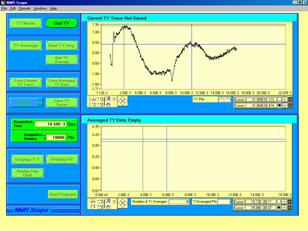
TY Mode

XY Mode

4. To stop the signal, press Quit TY, or Quit XY signal accordingly.

5. To save the data, press Save Current TY/XY Traces. Save the data as a .dat file format.

6. To clear the graph, press Clear TY/XY Traces.

Note: you can actually copy the graph and print it separately. Right click anywhere on the graph and press Copy Data. This temporary stores the image on the computer and you can paste it in most programs such as word or excel.

Averaging the Data:

We can also "average out" the signal to get a smother line. The program takes multiple samples over time and takes the average. You can average the data in wither mode: TY or XY. After choosing the mode, you might want to go over the following steps:

1. Press TY/XY Average. The window comes up asking if you want to "AutoSave the data." If you wish to do so, press yes and it will prompt you to save it. Otherwise, press no. In either case, you will get a window, asking to "Chose Acquisition Points." Just press ok. In the middle to the left of the program window you can set either the acquisition time or acquisition points. By default they are set to maximum.
2. Now, press Start TY/XY Average. The top right graph is the same as one before. The bottom right graph is the average graph. You might see similar graphs to the ones bellow:

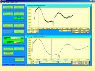
TY Mode

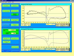
XY Mode

3. To stop the signal, press Quit TY/XY Average.

4. To save the data press Save Averaged TY/XY Data.

5. To clear the graphs press Clear TY/XY Traces.

Strip Chart Recording Function (used in the later part of the NMR experiment)

Instead of using the actual Strip Chart Recorder, we can use the NMR Scope program to accomplish the same results. Once all the equipment has been set up properly, the use of the program is simple.

1. Set up the equipment as instructed in the section "Taking Data," part E.
2. Open the NMR Scope program.
3. Press the button Display Strip Chart. You will see that you are only given one graph space in the top right corner.
4. To start taking the data, press Start Chart. You will see something similar to the following graph:
   
   

   
5. To stop the signal press Stop Chart
6. To save the data press Save Strip Chart
7. To clear the data press Clear Strip Chart

This concludes the overview of the program. If you have any more questions, you can ask one of the staff members for help.

 

9. NMR Pictures and Diagrams

     NMR head