Contents 1 Optical Pumping Description (OPT) 2 Optical Pumping Pictures 3 Before the Lab 4 Introduction 5 Preparation Before The Lab 6 Experimental Procedure 7 DS345 generator 7.1 The Effect of Temperature on Signal Strength 8 Analysis 8.1 Data Analysis 8.1.1 Overview 8.1.2 Nuclear Spins 8.1.3 Earth’s Magnetic Field 8.1.4 Errors in the Field 9 Notes and advice from Prof. Budker 10 References

Optical Pumping Description (OPT)

1. Note that there is NO eating or drinking in the 111-Lab anywhere, except in rooms 282 & 286 LeConte on the bench with the BLUE stripe around it. Thank You, the Staff.

This experiment is quantum mechanics in action. When a sample of gaseous atoms is placed in a static magnetic field, the electronic states undergo Zeeman energy level splittings in addition to fine structure and hyperfine structure splittings. By applying polarized light at the proper frequency, we can induce transitions from ground state levels to excited state energy levels. The atoms then decay to higher ground state levels until we have "pumped" all of them into the same (highest) ground state energy level. At this point we can see an increase in light passing through the sample because no more can be absorbed. However, when we apply a radiofrequency signal of just the right energy to stimulate transitions to a lower level, we see a sudden decrease in the radiation signal as the system is again pumped to the higher level. By determining the frequency of the RF signal we gain information about the atomic energy levels.

You will need to use your knowledge of fine, hyperfine, and Zeeman splitting to find the energy levels of two isotopes of rubidium. You will determine the nuclear spins of the isotopes, and the strength of the earth's magnetic field in the laboratory.

1. Pre-requisites: Physics 137B (may be taken concurrently)
2. Days Alloted for the Experiment: 3
3. Consecutive days: No

This lab will be graded 20% on theory, 30% on technique, and 50% on analysis. For more information, see the Advanced Lab Syllabus.

Comments: E-mail Don Orlando

 

---

Optical Pumping Pictures

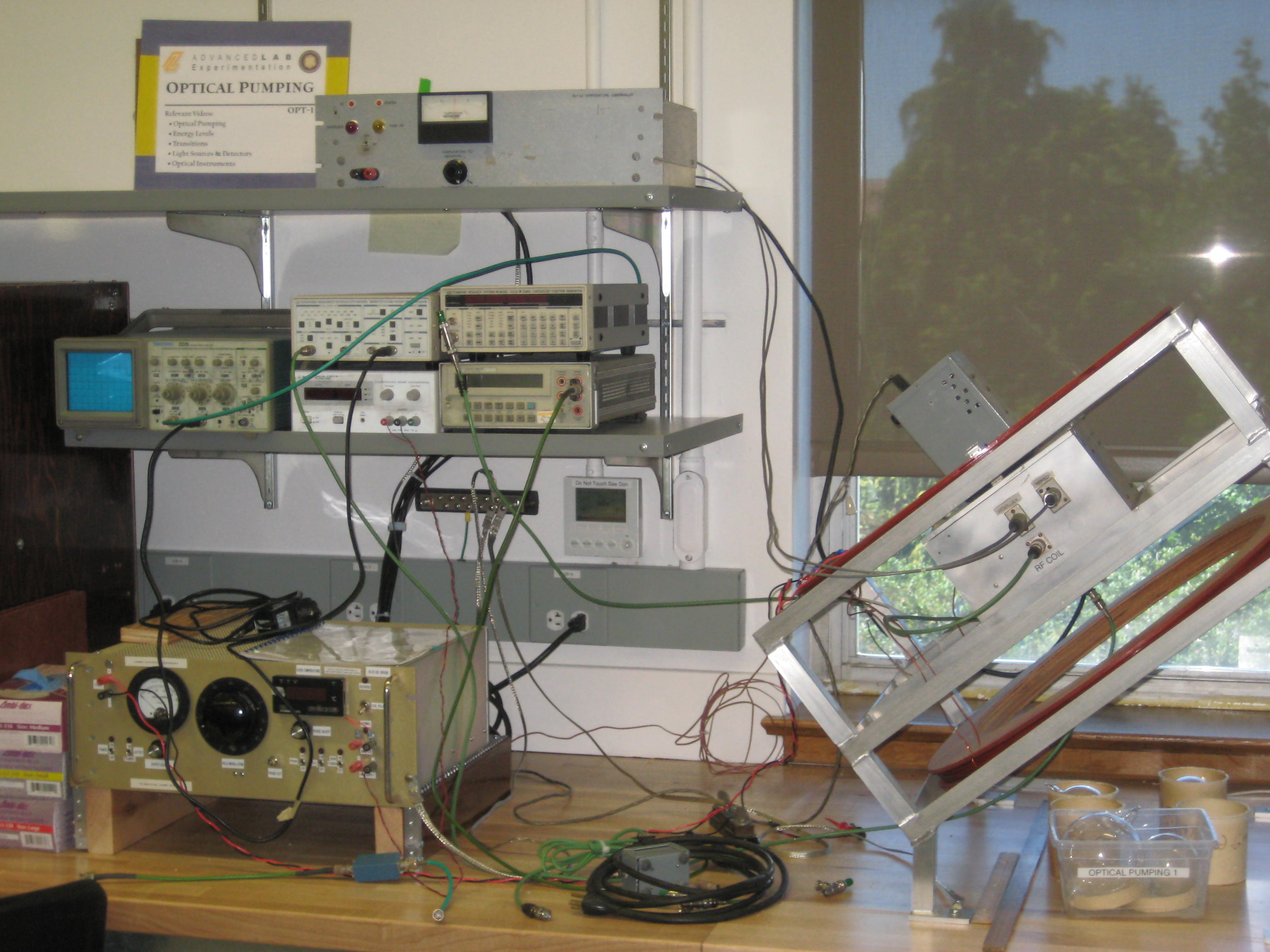Optical Pumping setup Click here to see larger picture

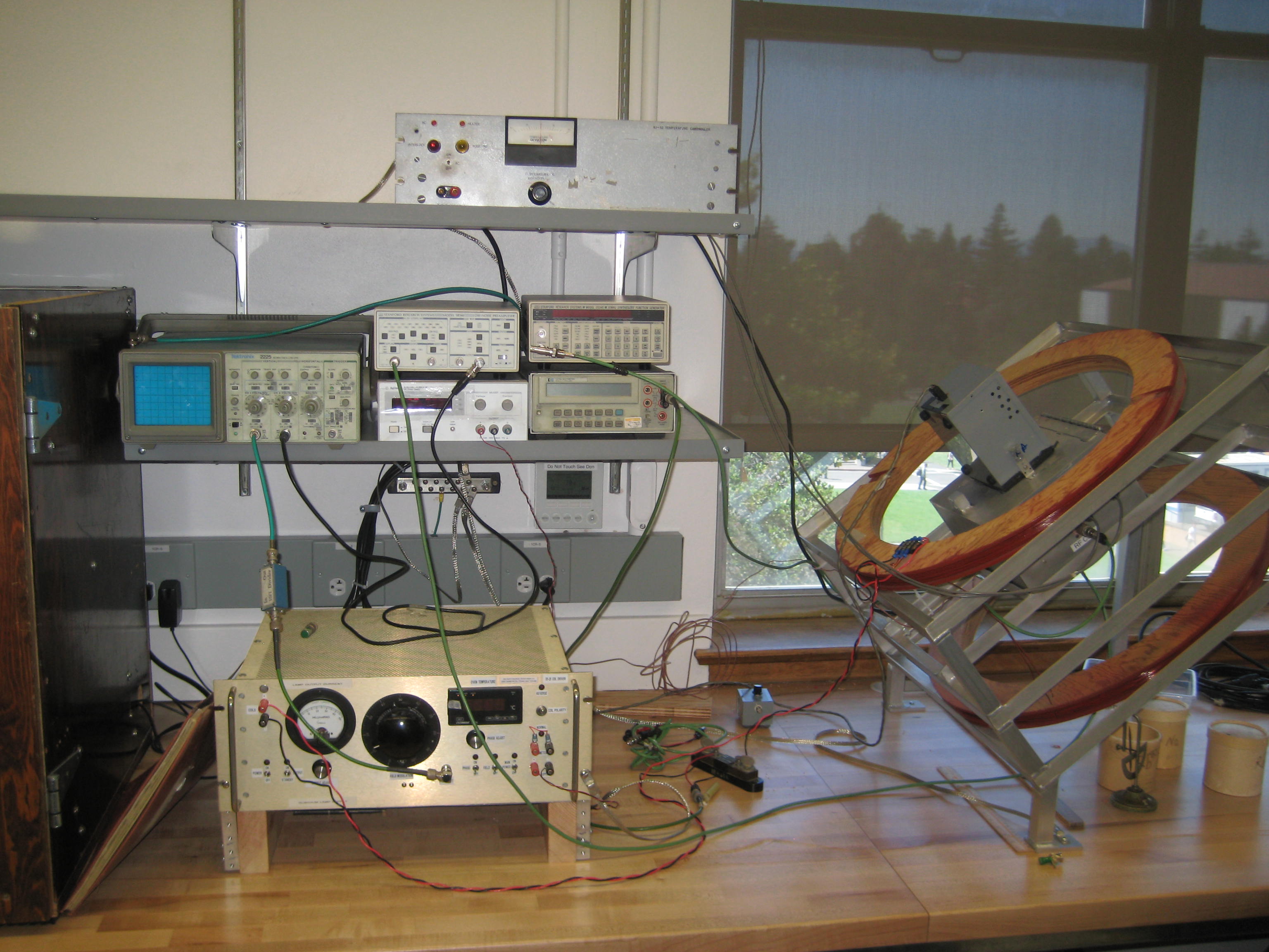Optical Pumping Equipment & Coil Click here to see larger picture

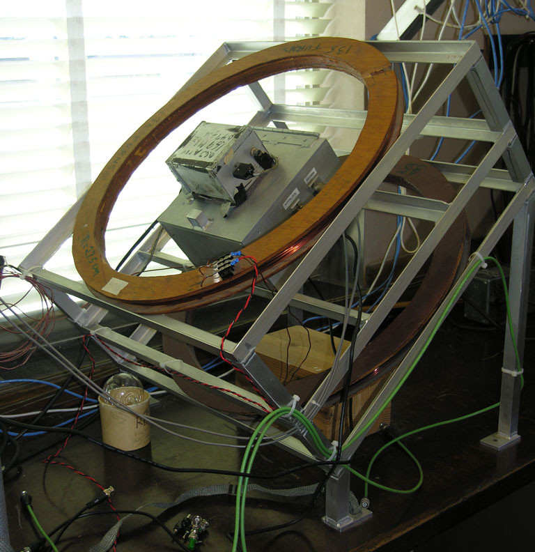
Optical Pumping coils assembly Click here to see larger picture

 

---

Before the Lab

Complete the following before your experiment's scheduled start date:

1. View the Optical Pumping video.

Note: While the OPT video has been a great resource for the students helping them to quickly orient in the lab, it has become apparent that some common misconceptions regarding the experiment stem from some minor inconsistencies in the video. To remedy this, I have compiled an (incomplete) list of corrections below labeled by the time in the video. On a personal note, I am sad that Prof. Sumner Davis, a wonderful warm person, a colleague of many years, and a 111 lab enthusiast is no longer with us to call upon to tweak the video…

Time code in Minutes for video in Bold:

05:26 The ²P_3/2 state splits into F=3,2,1, and 0 (because J=I=3/2 for ⁸⁷Rb).

06:30 The order of the M_F sublevels of the F=1 state has to be reversed (because g_F=-1/2).

12:34 The ratio of probabilities is not generally 50:50 (it depends on the specific sublevels involved), but this does not make too much of a difference for the discussion.

13:05 In the OPT experiment, the atoms are actually pumped into an |M_F|=2 sublevel of the F=2 state (in the case of ⁸⁷Rb).

14:53 I would say it is wrong to call radio-frequency radiation “light”.

18:02 It is incorrect to label the horizontal axis “t”.

20:22 The filter that removes the D2 radiation is not there to get rid of noise. In fact, if one removes the filter, while the same ground state will be pumped, the pumping, however, will not result in the rubidium vapor becoming transparent. This is a finer point of the experiment (of which there are many, most of them being glossed over).

2. Complete the OPT Pre Lab and Evaluation sheets. Print and fill it out. The Pre-Lab must be printed separately. Discuss the experiment and pre-lab questions with any faculty member or GSI and get it signed off by that faculty member or GSI. Turn in the signed pre-lab sheet with your lab report.

3. View the Error Analysis video.

Suggested Reading:

1. †R.L. De Zafra, “Optical Pumping”, Amer. Journ. of Phys. 28, 646 (1960). #QC1.A4 Searchable Page
2. Reference Rubidium Diagrams Rb Energy Levels
3. †A.L. Bloom, “Optical Pumping”, Scientific American, October 1960, p.72. #T1.S5
4. †N.F. Ramsey, Nuclear Moments, Wiley, 1953. #QC174.1.R31. Advanced treatment.
5. C.E. Moore. "Rubidium." Atomic Energy Levels Vol. II, National Bureau of Standards, 1952. #QC453.M6
6. Detailed description of an experiment on Electron Spin Resonance using optical pumping [Experiment setup]. Must read if you want to work out the first problem in the prelab.

More References

Physics 111-Lab Library Reference Site

Reprints and other information can be found on the Physics 111 Library Site.

You should keep a laboratory notebook. The notebook should contain a detailed record of everything that was done and how/why it was done, as well as all of the data and analysis, also with plenty of how/why entries. This will aid you when you write your report.

Introduction

Measuring the energy levels of atomic, molecular, nuclear, and particle systems is a large part of experimental physics. The technique of optical pumping is used to measure the difference between the atomic energy levels with great precision. This experiment uses optical pumping to measure the splitting of the rubidium atomic energy levels when the Rb atoms are placed in a magnetic field. It is so easy to make these measurements that you can use the opportunity to consolidate what you know and understand about atomic physics and quantum mechanics. You can get a solid appreciation of the physics and how elegant it is from this simple experiment. It also gives you an idea of how congested an actual laboratory set up is compared to how clean and organized the physics looks in a textbook.

Your goal in this lab is to find the resonance frequencies, and thereby measure the Zeeman splitting, of $^{85}$Rb and ^{$^{87}$}Rb for various magnetic field strengths. From this, you will then determine the nuclear spins of these isotopes and the strength of the Earth’s magnetic field.

Preparation Before The Lab

Starting with the articles by Bloom and de Zafra, read through the Optical Pumping Reprints. The reprints for this lab are all theoretical, and should be understood before coming to lab. Note, however, that not all of the diagrams or discussions are correct for our experiment: some of the articles discuss only transitions between hyperfine levels, while we have Zeeman splittings as well. Try to keep clear which splittings are which, and which are important for our transitions. See, for example, de Zafra (p.647). (You will also find that there is some variance in notation between the various reprint articles; parsing these differences can be challenging, but it is an important skill to have. Let the consistency of the base physics guide you.) As you study, here are some terms to understand:

absorption	electron configuration	linear and circular polarizers	radiative lifetime
atomic energy levels	equilibrium distribution	LS coupling	relaxation
atomic orientation	fine structure	magnetic dipole moment	resonance
buffer gas	Helmholtz coil	Maxwell-Boltzmann distribution	selection rules
Breit-Rabi equation	hyperfine structure	modulation	spontaneous emission
degeneracy	interference filter	nuclear spin	stimulated emission
discharge lamp	Larmor frequency	Paschen Bach effect	spectroscopic notation
electric dipole transition	line width	quantum numbers	Zeeman effect

A. Starting with the Hamiltonian

$ H = - \overrightarrow {\mu_I} \cdot \left ( \overrightarrow {B_J} + \overrightarrow {B_{ext}} \right ) - \overrightarrow {\mu_J} \cdot \overrightarrow {B_{ext}} $ (eq. 1)

where $ \overrightarrow {\mu_I} $ is the nuclear magnetic moment, $ \overrightarrow {\mu_J} $ is the electronic magnetic moment, $ \overrightarrow {B_J} $ is the magnetic field at the nucleus arising from the rest of the atom, and $ \overrightarrow {B_{ext}} $ is an externally applied field, derive the Breit-Rabi law in the low-field case:

$ \frac {\nu} {B_{ext}} = \left ( \frac {2.799} {2I + 1} \right ) \quad MHz / gauss $ (eq. 2)

(See Ramsey, for example. [Again, look for any notational differences that may exist; Ramsey lays out his conventions in the text, but some analysis may be required nonetheless.])

Also work out the numerical values of the g-factor associated with the split hyperfine states for ⁸⁵Rb and ⁸⁷Rb.

You will be asked to demonstrate this in the Pre-lab discussion, but you should not include it in your lab write up.

B. Derive the expression for the magnetic field at the rubidium bulb due to the Helmholtz coils:

$ 0.9 \times 10^{-6} \left ( \frac {tesla \cdot meter} {ampere} \right ) \frac {Ni} {a} $ (eq. 3)

where N is the number of turns of the coils, i is the current, and a is the radius of the coils. (Recall that there are 10⁴ Gauss in a Tesla.) Discuss the Helmholtz coil. Why is the field so uniform at the center, both laterally and longitudinally? How inhomogeneous is the magnetic field at the bulb? What are the qualitative and quantitative effects of this inhomogeneity? Are they important in this experiment?

You will be asked to demonstrate this in the Pre-lab discussion, but you should not include it in your lab write up.

C. What are the effects of the earth’s magnetic field? What would happen if the Helmholtz coils where not perfectly aligned with the earth’s field?

Experimental Procedure

Taking data for this experiment is more straightforward than for any other lab in this course. But the experiment deserves more time and thought than most because it illustrates fundamental ideas about quantum mechanics which you probably have only vague notions. Take the time to think about what’s going on, and answer any questions that occur to you. You should know the equipment and how this experiment is connected to make things work. We only give you a starting place you should change the gain and roll off on the amp. Check out the scope gain as well. Understand the signal flow for this experiment then it will be easy to complete.

 

1. Look over the block diagram (Figure 1) and check the connections of the equipment carefully (you need not hook up the oscilloscope or the [DS345] yet). Make sure you understand what each unit does and that you know the limitations of the equipment (e.g. don’t run the current of the coil higher than 3 A; be sure to understand how the voltmeter and shunt gives you precise current measurements; don’t drive the RF at more than 5 V; don’t heat the bulb over 50^o C; etc.) Inspect and open carefully the Rb light box to see its construction. Can you explain how the Rb lamp works? Be particularly careful of the D1 pass filter. It is expensive to replace! All pieces in this unit are already in their proper places. The large bulb filled with ⁸⁵Rb and ⁸⁷Rb should be in the light box. You should use different types of Rb bulbs to check the experiment if needed. The ratio of the two isotopes in the bulbs containing ⁸⁵Rb and ⁸⁷Rb mirrors the natural ratio.
   
   

   

   Figure 1: Block diagram of Equipment

2. Warning: Never turn off the plug strip if any of the equipment is powered up. Turn on all the equipment, starting with the Main switch (lower right-hand corner of the Rubidium Lamp Supply/Coil Driver Panel). Set the Rubidium Supply Output Current for the Rb lamp to approximately 25 milliamperes using the Adjust Knob. (Like much of the experimental apparatus, the Rb lamps at the two Optical Pumping stations are not identical; one may require a higher current to light the lamp at Station 2 [perhaps 30 milliamps].)
   
   

   

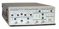
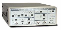
   Figure 2: SR560 Amplifier

3. When you turn on the [SR560 Voltage PRE-AMP] make sure that the INPUT ‘A’ is selected, the DC/GND/AC button is set to the AC position. To start, set the Gain to 500, LF Roll-off to 0.1 Hz, and the HF Roll-off to 10 KHz. You may have to change some settings to make your signal clear. Also note that if you suddenly lose your signal, i.e. if your scope trace goes to a flat-line, you should press the OL REC (OverLoad RECovery) button. The SR560 requires you to adjust the dynamic reserve and the filter roll-off; set the gain mode to low noise and the roll off to 6 dB per octave for both the high and low pass filters.
4. We will be using a DS 345 synthesized function generator to drive the RF coils in this experiment (see Figure 1). Before you begin taking data, it would be wise to familiarize yourself with its capabilities, its limitations, and its interface (see Figure 3 and the [DS345 Manual]).

DS345 generator

1. • You should start by looking at the output of the DS 345 on an oscilloscope. Connect the “Function” output of the DS 345 to Ch. 2 and drive it with a 5 V p-p, 5 kHz sine wave. (You can adjust the frequency by hitting the “Freq” button and then using the entry keypad [followed by V p-p] or the “Modify” arrows in conjunction with the step button to adjust the magnitude of the steps. Similarly, the amplitude can be set with the Ampl button.) Measure the amplitude of the signal on the scope; is it what the DS 345 claims to be outputting? You can use a BNC tee and a 50 Ohm terminator to terminate the output of the DS 345 and bring it closer to what is desired. (Note: DO Not Terminate the modulation output, this will damage the unit.) Considering how we will be using the DS 345 in this experiment, will it be important to have it produce a precise amplitude? Throughout this experiment, in order to avoid damaging the RF coils, you shouldn’t drive signals of much more than 5 V p-p, and you should terminate the frequency output to keep the DS 345 correct.
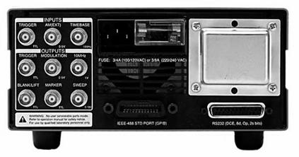
   • Try experimenting with the signal modulation capabilities of the DS 345 as we will use the 5V p-p sine wave which we have already set up as a “carrier” signal for frequency modulation (FM). Start with running a BNC cable from the modulation output (Do Not Terminate) of the DS345 (on the back panel, see figure 3) to the Ch. 1 (X) input of the oscilloscope and connect the terminated function output of the DS 345 to the Ch. 2 (Y) input of the scope. Set the oscilloscope to trigger off of channel 1 in the “Norm” mode. Set the scope to “Alt” rather than “Chop”. First, try amplitude modulating the 5V p-p 5 kHz sine wave (the carrier signal) with a 500 Hz square wave. The frequency of the modulation is set using the “Rate” button; the modulation can be turned on and off using the “Sweep” button, and the shape of the modulation function [square, sine, etc.] is set using the second set of arrows in the Sweep/Modulate panel. The depth of modulation can be adjusted with the “Span” button; for AM modulation, the span is a percentage (0-100) of the carrier (unmodulated function) amplitude. Start with setting the span to 100. Looking at the output with a dual linear sweep, what do you see? What is the maximum amplitude of the Function output? How does it compare with the unmodulated amplitude? Experiment with different modulation waveforms, span, and rate settings. You might also try using the X-Y mode of the scope to observe the output of the DS 345 (Function output against Modulation output) but don’t let it confuse you. It is important to have a clear understanding of what the X-Y mode represents and when to use it (the display is called a Lissajous figure). In the X-Y mode, the oscilloscope no longer displays a time axis. The voltage amplitude for an input is displayed on the respective axis. (See the XYZ’s of scopes at the BSC stations)
   • Note that the modulation output is just a 0-5 V representation of the modulation function (Do Not Terminate Modulation output) as described in the DS 345 Manual. If “sweep” is on, the modulation output will always vary between zero and 5 V, regardless of the size of the actual span. In other words, it is a relative indicator. (With AM modulations, the modulation output will always be zero when the function amplitude is at a minimum and 5 V when the function amplitude is at a maximum [2.5V would then correspond to the amplitude of the unmodulated carrier].)
   • Now try frequency modulation. Give the 5 kHz, 5V p-p sine wave, carrier signal a 500 Hz square wave FM modulation. As with AM mode, the rate of the modulation (the frequency of the modulation signal) is set with the “rate” button. In FM mode, the span button sets the peak-to-peak frequency shift that occurs in a modulation cycle. Set the span to 8 kHz; the frequency of the function output should shift between 1 kHz and 9 kHz. Note that you can’t set the span to twice the carrier frequency or more (the DS345 has trouble making oscillations with zero or negative frequencies). Try different modulation waveforms; look at sine, triangle and ramp modulations. Again, start with the oscilloscope in the linear, time sweep mode. The X-Y mode can also be revealing if you keep in mind what the modulation output represents. (As with AM, in FM, the modulation output gives a 0-5 V representation of the modulation function. Again, zero volts corresponds to the minimum frequency [the carrier frequency minus half the span] and 5 volts corresponds to the maximum frequency [the carrier frequency plus half the span], and so forth.) You should now have familiarised with the DS345 enough for this experiment.
     
     

     

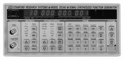
     Figure 3a: DS 345 Synthesized Function Generator (Front)

     

     

     Figure 3b: DS 345 Synthesized Function Generator (Back)

2. Heat the sample to 48 ^oC, then turn the heater off to reduce noise, (noise due to what?) but remember that you want the temperature between 38 ^oC and 45 ^oC for good data. (Why? See Optical Signal vs Temperature) A reading from the temperature sensor is output to an LED display labelled 'Oven Temperature'. Make sure the temperature does not go above 50 ^oC; if you start to approach this temperature, turn down the thermostat. The heater has an overtemperture shutoff switch in the heater box. If you overtemperture the box it will need time to rest and you should call one of the staff.
3. We will now attempt to roughly observe the variation in the opacity of Rubidium gas that occur when it is optically pumped and then hit by the resonance frequency RF by applying a variable frequency signal. We will look at a wide range of frequencies so that we will be sure to see resonance effects for both isotopes.
   • Connect the function output of the DS345 to the RF coils. Set the DS345 to output a 3 MHz sine wave with a 10 Hz, ramp function FM modulation. (Use the “Freq” button to set the carrier frequency to 3 MHz; use the “Rate” button to set the modulation frequency to 10 Hz.) Set the span of the modulation to a little less than twice the carrier frequency (5.9999 MHz). Try setting the DS 345 Span to 6 Mhz. Why does it give an error? See DS345 Manual: FM Modulation section. Connect the photo diode's output to the PRE-AMP and make sure the PRE-AMP settings are as specified before. Run the output of the PRE-AMP (the amplified photodiode output, see [Photodiode Data Sheet] for photodectector operation) to Ch.2 (Y) of the oscilloscope and keep Ch.1 (X) connected to the DS 345’s modulation output. Set the oscilloscope to X-Y mode. (See the Photodiode Data Sheet for details on the photodetector’s operation)
   • Turn on the HP E3615A DC power supply. (We want a DC field at this point; check that the field switch on the coil driver is off.) Set the coil current to one amp 1.0 Amp (Note you may need to change the current to find the signal).

Use the Current knob on the Power Supply to adjust the current and the shunt to measure it. The shunt is a calibrated resistor and is temperature compensated. The voltage that develops across the shunt is 10mV per Amp of current through the coils. The Digital Volt meter reads the milivolt reading. (Note that there is a button on the front of the Digital Volt meter that changes the connections from front to rear of the unit.) This button should be in the front position. On the oscilloscope, you should see something like what is shown in figure 4. (You may see some 60 Hz noise in your signal; adjusting the connections may help minimize the problem.) Explain what you see. Make sure you understand what the scope, in X-Y mode, is showing. What do the axes represent? Make an approximate measurement of the two resonant frequencies. Again, keep in mind that the span gives the peak-peak frequency variation, so the modulation output should be varying from ~0 to ~6 MHz. If you set the Ch1 [X] scale to .5 V/div, then the signal sweeps out exactly ten divisions. Each division would then correspond to a change in frequency of 0.6 MHz, with the far left end of the range [corresponding to 0V] being at roughly 0 MHz. To get a more accurate measurement of the resonance peaks, adjust the carrier frequency of the FM and narrow the span. This can be done successively to yield a reasonably accurate result. Which resonance is stronger? Which isotope does this resonance correspond to (the natural abundances of the two isotopes might provide a clue)? This information can be found on the nuclide chart. What happens to the signal as the temperature is varied? Do the relative strengths of each resonance change? Now try varying the current; go from zero to two amps in both the forward and reverse directions. What happens to the resonance frequencies and the size of the corresponding voltage changes? Are there any values of the coil current for which there is no resonance? What happens at zero current? Try adjusting the span, rate, and carrier frequency, and using a triangle rather than a ramp modulation.

1. In order to measure the resonance frequency more precisely, we will look at how the amplified light from the photodetector varies with a 60 Hz modulation in the magnetic field. That is, we will modulate the coil current and not the RF. Turn off the modulation on the DS345 (you may want to change the frequency of the carrier so it is closer to the resonance. The magnetic modulation does not cover as much as the RF modulation did so you might want to set the new frequency to a value that is close to the frequency value. But do not worry to much a rough estimate will work). Turn on field modulation by flipping the “Field” switch on the Coil Driver panel , and turn on the “Phase Out” output with the “Phase Switch.” Why do you think we use a 60 Hz modulation?
   • Familiarize yourself with the Coil Driver panel. The PHASE ADJUST control on Coil Driver panel changes the phase of the modulation signal seen by the scope (the Phase Out signal) relative to the modulation signal seen by the rubidium sample (that is, the actual modulation in the coil current on whose phase the photo-detected signal should depend). To examine how it works, feed the Phase Out (field modulation) signal through the divide-by-ten attenuator to Ch 1 (X) of the oscilloscope and feed the amplified photodetector signal (the PRE-AMP output) to Ch 2 (Y). With the scope in Dual Trace Mode (Both Channels), trigger on EXT/Line Source (60 Hz PG&E power line) and set the time scale to around 2 msec/DIV. You may have to adjust the trigger Level knob to get a stable trace. Now change the phase with the Adjust knob: the modulation signal (Ch. 1) moves because we are changing its phase relative to the 60 Hz line signal that we are triggering on. The detected signal does not, though, because the Adjust knob does not change the phase of the signal that the sample sees.
2. Put the scope in X-Y mode. You should now see the detected signal (Ch. 2) displayed on the y-axis versus the field modulation signal (Ch. 1) on the x-axis. How you can tell when you have found the resonance condition in this mode? Should there be any symmetry? If so, how should it be symmetrical? Along what axis should the symmetry be found? Consult the reprints. They have many useful figures to help you understand the relationship between the displayed signal and the conditions of resonance. It is up to you to determine which of the modes (Time Trace or X-Y) gives a more precise determination of the resonance condition–you might consider using both. Try them for repeatability. Estimate your errors using each method.
3. Refine the resonance frequency measurements that you made previously. Set the DC coil current to 1 Amp, as before, and, with no modulation (sweep off) vary the RF frequency about the stronger of the two resonances you found in part F. (Start by setting “freq” to the resonance frequency estimate you got in part F, then adjust it by relatively large increments [step size = 10 kHz], until you see a shift in the signal, then hone in on resonance with ever decreasing step sizes until you have it precisely.) Set the Field Modulation Powerstat knob to around 10 (relative scale). Take care not to set the modulation amplitude so large that you see resonances of both isotopes simultaneously (if this is possible). Make sketches of what the resonance signal looks like with proper and improper adjustments of modulation amplitude and phase; to get a sense of what setting for the phase is appropriate, you might check the appearance of the signal with a dual linear sweep. If you can’t find a resonance, get help. (You could search for resonance by setting the frequency to some fixed value and then varying the coil current. The oscilloscope pattern would look exactly the same.)
4. Once you have found the resonance condition; vary all of the parameters – current, voltage, temperature, phase, and whatever variables are under your control to get an idea of what the signal looks like under various conditions. How sensitive are your resonance measurements to changing variables? Record the qualitative behavior, and explain it. You should also get a quantitative estimate of the statistical error in you measurement technique; try making several independent measurements of the resonance frequency and see how they vary (See the Error Analysis Notes for further discussion of errors). Are there any possible sources of systematic error? You may want to check that the field is properly aligned; find the field direction meter (vertical compass) and place it close to the center of the Helmholtz coils. See what happens to the magnetized “needle” when you reverse the current or turn off the power supply. You should also get a sense of what effects 60 cycle pick up might have on your measurements.
5. You can measure the pumping time at resonance with a square wave amplitude modulation. Turn off the field modulation (field switch) but keep the coil current set to 1 Amp and the function (carrier) frequency set to the frequency of the stronger resonance that you measured. Keep Ch.2 of the scope connected to the PRE-AMP, and run the modulation output of the DS345 into channel 1. Again, make sure that you keep the temperature in the right range, but take data with the heater off. Set the DS345 to amplitude modulate the resonance frequency signal with a depth of 100%. With the scope in linear mode, adjust the modulation rate so that the gas reaches equilibrium before each shift in RF amplitude. Measure the rate of change in the signal height when the RF is gated on or off (that is, when the modulation signal goes from low to high or from high to low). (The time for the signal to change by 1/e is a good number to get.) Which corresponds to the pumping time and which to the relaxation time? To get a good measurement of the pumping and relaxation times, try using “Norm” triggering on Ch.1. You should also take advantage of the scope’s magnification capabilities. (The horizontal mode can be set to Mag, with magnifications of x5, x10, and x50.) You may see a lot of 60 cycle pick up in you photodiode signal; you might try adjusting the co-ax line from the photodiode to the PRE-AMP to minimize this. You should also be mindful of the effects the PRE-AMP’s filters and source coupling can have on your signal; adjust them to make sure that your values are real. Try looking at the resonance for the other isotope. Are the time constants the same?
   • If you observe the relaxation process with a high enough magnification (say x50 at 20 sec/div) you will see small oscillations in the signal even after you eliminate 60 cycle noise. These are real, physical effects in the relaxation process known as Rabi oscillations. (You should be able to distinguish them from noise by modulating the frequency by small increments, [less than 1 Hz, say]; if they continue to track with the modulation, they’re probably real.)
6. We will now use coil current modulation (as in part I) to measure the resonance frequencies for both isotopes over a range of currents. Keep Ch.2 of the oscilloscope attached to the PRE-AMP output and run the Phase Out (field modulation) output to Ch.1, and use X-Y mode. Starting at zero current, the two curves can be found near 200Khz and 300Khz. Starting at 2 amps, the resonance points can be found near 4.31 Mhz and 6.48 Mhz. The best way to take this data is to find a resonance point at either zero or 2 amps and follow it up or down the frequency spectrum by making small adjustments to both the current and the frequency. Again, steps of 10Khz works well. The goal is to keep the resonance pattern on the scope as to not lose it or worse jump to the other isotope’s resonance curve. Take at least 10 data points in increments of approximately 0.2 amps over the range of 0-2 amps for both isotopes in both normal and reverse current directions. That means four sets of data. You can take both current directions simply by revering the polarity at each step of current and refine the tuning of resonance. You should have an estimate of the error for the frequency and current measurements. Derive a method for determining this error with your lab partner utilizing the Error Analysis Notes. Discuss this method with a GSI Before Taking Data. You need not repeat Section J for every measurement, but you should get a representative sample that at least includes both isotopes (the isotopes have different intensities, so one might expect different error values). It should be possible to get fairly accurate and precise resonance measurements using small span RF frequency modulation (as in part L); if you have time, you might try retaking your points with this alternate methodology.
7. Turn off the RF generator, and vary the current while looking for a resonance. The field should be on with reverse polarity. Set the field modulation to 10. Set the oscilloscope for a linear internal sweep in the x-direction. The resonance should be found around 0.08 A.( This is known as the Zero Field Resonance.)

 

The Effect of Temperature on Signal Strength

Note: Temperatures for ⁸⁷Rb may be different. Why? (Note that ⁸⁷Rb signal peaks at 42^oC)

Analysis

(See Error Analysis Notes for further discussion.)

1. Make plots of frequency vs. current to help you analyze your data. You should have four sets of data and four lines when you plot them. The individual points, the slopes of the curves, and their axial intercepts have an interrelated significance.
2. You have two equations to work with; one is the Breit-Rabi equation (eq. 2), and the other is the field of Helmholtz coils as a function of current (eq. 3). Write down the equations, rearrange them, see how the two isotopes fit in, see how additions or subtractions can help, use both + and – currents. Keep in mind that the B-field in the Breit-Rabi equation is the sum or difference of the field of the Helmholtz coils and the Earth’s field. From equation (2) we have a relation between $ \nu_1 $ and I₁, and $ \nu_2 $ and I₂ where the subscripts refer to the Rb⁸⁵ and Rb⁸⁷ isotopes. From your data determine the best ratio $ \frac {\nu_1}{\nu_2} $ and from this deduce the values of I1 and I2. Their true values are exactly half-integral. (Are the ratio, and this half-integral expectation, sufficient to determine both nuclear moments?)
3. Having now determined the values of I₁ and I₂, use equation (2) to determine the value of B at the bulb for one positive and one negative value of the current in the coil. Compare these values with those calculated from the coil dimensions and current. Which values are more accurate? Why? Once you have determined the nuclear spins, the Breit-Rabi equation is as accurate as the numerical constant 2.799, since the nuclear spins must be odd half-integers exactly. The field of the Helmholtz coils is not as accurate as the numerical constant 0.9x10^-6 since the radii of the copper wire turns are not all exactly the same, and the separation of the coils is not exact. By using the Breit-Rabi equation, you can determine this constant more accurately. Try drawing a line parallel to the frequency axis at a particular current, both plus and minus. What can you learn from the intersections with the curves? Do the same with a line parallel to the current or B axis.
4. Perform a line fit on each of your four data sets. For each, find the slope and intercept and there respective errors using the theory and techniques of error analysis as illustrated in Lyons, Data Analysis for Physical Science Students, Section 2.9, page 63ff. (Also see Error Analysis Notes). Show clearly how you do this, with a sample calculation. If you use Excel you must show that you know what the program is doing. In particular, what is R and what influences its value? Don’t just use a data reduction code blindly – you don’t learn anything that way. You might also try a Chi-Square analysis to check whether your data and error estimates are consistent (again, see Lyons). Also, check to see that their slopes are consistent with the values of nuclear spins that you found.
5. From the intercepts calculate the earth’s field, and its errors. Ultimately you can have four values for the earth’s field for each isotope. Check to see that all eight values fall within the range of your statistical errors. If they don’t, what might be wrong? Say something about which values you think are the most accurate, and why.
6. Explain why there is a resonance at zero field, i.e. the magnetic field generated by the Helmholtz coils and the Earth magnetic field sum up to zero.
7. What do you need to know and to take account of, in order to make a rough estimate or calculation of the pumping time to compare with your experimentally measured value?
8. Go to the page on data analysis and complete the steps.

 

Data Analysis

Overview

The purposes of the experiment are

1. to determine the nuclear spins of the two isotopes ⁸⁵Rb and ⁸⁷Rb. It is known that both spins are odd half-integral values, like 1/2, 3/2, 5/2, etc., and
2. to measure B_e, the Earth’s magnetic field.

We have two rubidium isotopes in gaseous form inside a bulb placed in a magnetic field and subject to electromagnetic radiation. The Earth’s magnetic field also affects the rubidium energy levels and their populations. We set the current in the coil producing the magnetic field, and adjust the radio frequency to produce a resonance condition. The parameters that we either want to change, vary, or to measure are the current, the field produced by the current, and the frequency of the applied RF radiation at resonance. The relevant equations are:

$ 0.9 \times 10^{-6} \left ( \frac {tesla \cdot meter} {ampere} \right ) \frac {Ni} {a} $

B_H, magnetic field from the Helmholtz coils

i, current in the coils

a, radius of the coils

The value 0.9 is approximate because the radius a is not exactly the same for each of the N windings and we have no simpler way of incorporating this fact.

$ \frac {\nu}{B_{ext}} = \frac {2.799} {2I + 1} \quad MHz / gauss $

ν, frequency of applied em radiation

I, nuclear spin of Rb

B = B_H + B_e, the total magnetic field from the Helmholtz coil and the Earth

This equation is called the “Breit-Rabi” [bright-robby] equation.

Nuclear Spins

How and what data should you take? To determine the nuclear spins, rearrange the equation to get an equation that looks like y = mx + b. Then set a value of the current i, adjust the RF to the resonance value, reset i, etc., until you have a table of pairs of values. In fact, you will end up with four tables, because you should take data for both positive and negative currents for each of two isotopes. A plot of resonance frequency vs. current will give a straight line with a slope dependent on 2I + 1, and an intercept dependent only on the earth’s field. [Sketch 4 straight lines]

Another way of determining the spins is to set the current and take the ratio of the resonance frequencies for the two isotopes, at the same current.

In both methods there will be some errors, but it does not matter because we know that the spins have exact half-integral values. This is a case in which the use of error analysis is unwarranted because the results are unambiguous.

Earth’s Magnetic Field

To determine the value of the earth’s magnetic field, we need to find a way to determine B_H exactly, or to eliminate it from the equations. B_H can be eliminated by setting i = 0 and using the frequency intercepts and the Breit-Rabi equation. Recall that the equation for B_H as a function of i is not exact.

There is yet another way to determine the earth’s field. There is a reversing switch on the coil current, to reverse the direction of the field. For the same absolute value of the current, the field must have the same strength, except for possible hysteresis effects. Check for hysteresis by measuring the resonant frequency at a particular current, when the value of current is reached from above (run the current to a max, and then come down to the desired value), and from below (run the current to zero, and then come up to the desired value).

So, at a particular current, measure the resonance frequencies for both positive and negative values of current. Add and subtract the two equations, and get exact expressions for B_e and for the more exact parameter for the relation between current and B_H.

Errors in the Field

How do we treat the errors in the value of the earth’s field? Step back a little, and see what data you have and how you can arrange it to make error computation the simplest. Here are several approaches.

1. Look at plots of your data. You should have 4 lines, two for each isotope, one with positive current and one with negative current. You can do a least-square fit of each line, calculate the position of the zero-current intercepts, and obtain values for the field. Then you can calculate “errors of adjusted coefficients” using the methods given in Lyons and other references.
2. But, by changing negative current points to negative frequencies as well, each isotope has only one plot line and presumably the zero crossing is more accurate. Then there are only two lines to fit, one for each isotope, and the errors can be calculated as described above for adjusted coefficients.
3. A still easier method is to use pairs of points with the same absolute values of current, and add the two resulting equations. We then have values of the earth’s field without adjusting any coefficients, and the errors can be calculated as an error of a single parameter, rather than as an error of an adjusted coefficient. We have

$\nu^+ =\frac{2.799(\overrightarrow{B_H} | + | \overrightarrow{B_E} |)}{2I + 1}$

$\nu^+ =\frac{2.799(\overrightarrow{B_H} | - | \overrightarrow{B_E} |)}{2I + 1}$

$|\overrightarrow{B_E}| = \frac {1}{2} \left ( \frac { |\nu^+ - \nu^-|}{2.799} \right ) \left ( 2I + 1 \right ) $

The standard deviation is calculated as described above in Error of a Single Parameter: Measurement Statistics. Compute the average; compute the differences, square them, add, divide by N(N - 1) and take the square root. Then step back, look at the results, and see if they look reasonable. If not, you’ve goofed somewhere, and must try again.

Notes and advice from Prof. Budker

• Nov. 19, 2007. The Physics-111 Optical Pumping experiment utilizes radio-frequency transitions between Zeeman sublevels split in energy in an external magnetic field (for example, the field of the Earth). The experiment illustrates how an optical-pumping device can be used as a magnetometer. Another interesting and very important application of optical pumping is atomic clocks. The clocks are based on microwave (rather than rf) transitions which are between the two ground-state hyperfine-structure levels (i.e., the levels with different total angular momentum F). A nice discussion appropriate for the Physics-111 students (particularly those who have mastered the Optical Pumping experiment) is given in an article by James Camparo, "The Rubidium Atomic Clock and Basic Research," Physics Today -- November 2007.
• Here, I plan to list some common misconceptions about OP.

 

References

1. J.R. Taylor, Taylor Book 2ed "An Introduction to Error Analysis", Oxford,
2. L. Lyons, "A Practical Guide to Data Analysis for Physical Science Students", Cambridge, 1991. #QC33.L9
3. James Camparo, “The Rubidium Atomic Clock and Basic Research”, Physics Today -- November 2007
4. Carver, Thomas R. "Optical Pumping"; Science: vol. 141, Aug 16, 1963, pp. 599-608.
5. Corney, Alan, "The Hanle Effect and The Theory of Resonance Fluorescence Experiments"; Atomic and Laser Spectroscopy, (1977). Pp. 473-533.
6. Diagrams of the electronics [Diagrams]
7. Check out all the Reprints for this experiment;
8. [Data Analysis Books] on Physics 111 library site

Other reprints and reference materials can be found on the Physics 111 Library Site